## I. INTRODUCTION Today, with the expansion of IoT devices, one of the most significant challenges is developing a communication theory that can reduce the power consumption of the nodes while maintaining a long communication range. In the last decade, different technologies have been proposed for this purpose. Recently, LPWAN technology such as LoRa, SIGFOX, and NB-IoT has been seen as a promising candidate for future IoT applications [1-5]. However, with extremely low power requirements in today's IoT applications, active communication using power hungry devices such as amplifiers, filters, and oscillators is limited. These small objects are sometimes placed in environments where battery replacement or recharging is difficult. Therefore, backscatter communication has been seen as a promising solution to significantly lower power consumption by communicating with nodes using passive devices [6]. Backscatter communication has been widely used for different low-power applications such as environmental monitoring, health monitoring, and localization [7, 8]. One of the advantages of backscatter technology is its ability to rely on available ambient RF signal sources in the environment, such as FM and TV broadcasting, WIFI, or cellular signal [9-12]. This significantly lowers the deployment cost since any dedicated signal source is required as in bi-static backscatter configuration. Several ambient backscatter communication systems have been proposed in the literature. In [12], the ready available FM broadcasting signal is used to backscatter tag data that can be decoded in any FM receiver. In that work, a range of 60 feet (18.2 m) was achieved and consuming only 11.07 W of power. [11] uses Wi-Fi transmission as an excitation signal to backscatter tag information to be decoded by a Wi-Fi access point. They achieve a communication rate of 5Mbps at a range of 1m and 1Mbps at 5m. In work [13], the maximum range for backscatter communication utilizing the ambient FM radio signal was presented. Using a ray-tracing technique and radar equation, and placing the receiver antenna close to the FM transmitter as in monostatic backscatter, a distance of 14.5 km was achieved. The limited range of technologies mentioned above has motivated the research community to develop a backscatter system that uses LoRa transmission as an excitation signal. The high sensitivity of the LoRa signal due to CSS-type modulation has been used by researchers to develop the LoRa backscatter communication technique for energy-constrained IoT devices communication [14-18]. LoRa backscatter is intended to improve communication range while consuming a small amount of energy. For example, [16] overturns the conventional short-range wisdom of backscatter and presents a LoRa Back system that can transmit up to $475\mathrm{m}$ and consumes only $9.25\mu W$ of power while being compatible with commodity LoRa hardware. The error performance of LoRa backscatter has been addressed in the literature. In [19], a closed-form expression was derived for SER on both the AWGN and the Nakagami-m double fading channels. The authors in [20] propose a receiver design based on the square-law detector to theoretically evaluate the error performance of the LoRa backscatter system under the AWGN channel and derive an approximate closed-form expression of the bit error rate using the union bond method. The authors show that LoRa backscatter outperforms active LoRa for SNR values between 2 and 9 dB. The authors in [21] present a comprehensive review of the literature on LoRa backscatter technology with an emphasis on tag design, interference cancellation techniques, receiver design, applications, and future research directions. Despite the broad literature, the link budget of LoRa backscatter is not adequately addressed yet. We aim to evaluate the communication channel using a path loss channel model to derive the transmission range between the LoRa backscatter tag and the receiver. In this paper, we propose an analytical model to evaluate the propagation channel and estimate the communication range between the tag and the receiver in different propagation environments. The proposed model can be used to optimize network efficiency. Our key contributions to this work are summarized as follows. - We develop an analytical model to estimate the communication range of LoRa backscatter technology. The proposed model can be used to theoretically estimate how far a receiver can be placed from the tag based on the design parameters such as the modulation scheme, the properties of the tag material and the propagation environment. - Analyze the effect of different parameters that affect the communication range, such as active LoRa parameters, the propagation environment, and antenna polarization. - We have extended the model to account for the effect of inter-tag interference, time, and frequency synchronization as well as the near-far problem for a concurrent transmission where several tags concurrently transmit to a receiver simultaneously. - Evaluate the accuracy of our range model by comparing it with the achieved range in state-of-the-art LoRa backscatter systems that use proof-of-concept prototypes. The remainder of this paper is structured as follows. In Section 2, we present the principles of LoRa backscatter communication. Section 3 develops a theoretical model for estimating the range between the RF tag and the receiver in LoRa backscatter communication with details of each parameter. Section 4 presents the simulation results and discussion. The work was concluded in Section 5. ## II. OVERVIEW OF LORA BACKSCATTER LoRa backscatter technology is an ambient backscatter communication technique that uses an ambient LoRa signal as an excitation signal. Depending on the type of excitation signal, two possible LoRa backscatter designs are possible: first, the excitation is an unmodulated single tone that a backscatter tag uses to synthesize a LoRa compatible packet and transmit information to the receiver [16, 17, 22-24]. However, this requires complex tag operation and hence increases its energy consumption. The second idea consists of using the LoRa-modulated signal to encode the tag data and backscatter to the receiver [14, 15, 18]. This type of tag design is complex because of the cancellation of the interference from the LoRa transmitter, which is complex and unknown to both the tag and the receiver. To address this challenge, the work [18] simply shifts the excitation signal to another channel and therefore creates out-of-band interference that limits network performance. [15] shifts the excitation in the same band as the backscatter signal and proposes a method to combine the energy in double sidebands to enhance the SNR. Using an ambient LoRa signal as excitation requires the tag to detect its presence and pick it from unwanted signals. This is achieved using a packet detection circuit. The packet detection circuit in the LoRa backscatter tag is characterized by its power consumption and sensitivity. The higher the sensitivity, the higher the distance from the source to the tag. ## III. PROPOSED MODEL In this section, we present the step-by-step derivation of the proposed model using the path loss channel modeling for different propagation environments. Path loss channel models represent the power reduction of a transmitted signal as it traverses the wireless medium. These channel models are based on the medium through which the signal travels, such as free space, rain, fog, or gas. We will derive a range estimation model for free-space and realistic scenarios of LOS and NLOS. The flow chart of the proposed model is illustrated in Figure 1. At first, a single node communication is considered, where one transmitter communicates with one receiver. 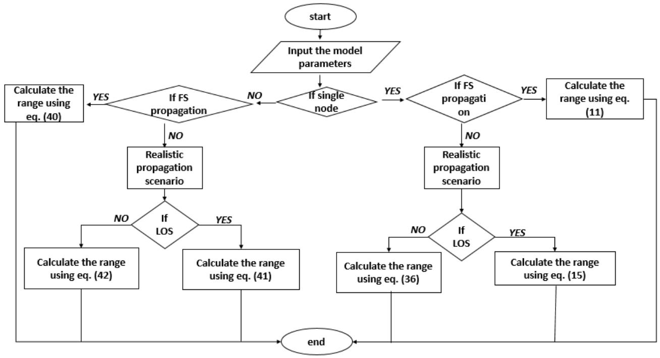If the propagation channel is the free space environment, the theoretical  Figure 1: Flow Chart of the Proposed Model Derivation range is calculated using eq. (11). For a realistic scenario, the impacts of different losses are considered. The eq. (15) and eq. (36) are used to calculate the range of the tag and the receiver for the LOS and NLOS scenarios, respectively. When multiple nodes are deployed in the network, communication from different nodes will introduce interference that affects link quality. Similarly, the communication ranges that account for the effect of interference are calculated for free space, LOS, and NLOS using eq. (40), (41), (42), respectively.  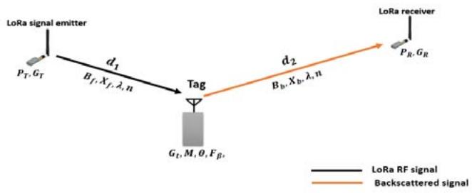Figure 2: System Overview of Ambient Lora Backscatter a) Free Space Propagation In backscatter communication systems, the link can be divided into two parts, i.e. the forward (unmodulated) and backward (modulated) links, as shown in Figure 2. The link budget for the forward link using the Friis free space equation is given as [25]: $$ P _ {t} = P _ {T} G _ {T} G _ {t} M \left(\frac {\lambda}{4 \pi d _ {1}}\right) ^ {2} \tag {1} $$ $P_{t}$ is the received power at the tag location, $P_{T}$ is the transmit power, $G_{T}$ and $G_{t}$ are the transmitter and tag antenna gain respectively. $d_{1}$ is the distance between the transmitter and tag, and $\lambda$ is the wavelength. M is the modulator factor and will be more detailed in Section 3.3.1 Similarly, the link budget for the backward link is defined as- $$ P _ {R} = P _ {t} G _ {R} G _ {t} M \left(\frac {\lambda}{4 \pi d _ {2}}\right) ^ {2} \tag {2} $$ Where $P_{R}$ is the received power at the LoRa backscatter receiver, $P_{t}$ is the received power at the tag, and $G_{R}$ is the receiver antenna gain. $d_{2}$ is the distance between the tag and the receiver. We can derive the free space path loss for the forward and the backward link from Eq. (1) and (2) as- $$ P _ {f} ^ {F S} = \frac {P _ {T}}{P _ {t}} = \frac {\left(4 \pi d _ {1}\right) ^ {2}}{G _ {T} G _ {t} \lambda^ {2}} \tag {3} $$ $$ P _ {b} ^ {F S} = \frac {P _ {t}}{P _ {R}} = \frac {\left(4 \pi d _ {2}\right) ^ {2}}{G _ {R} G _ {t} M \lambda^ {2}} \tag {4} $$ Multiplying Eq. (3) by Eq. (4) results in combined path loss for the free space the backscatter link and is given as- $$ P _ {c} ^ {F S} = \frac {P _ {T}}{P _ {R}} = \frac {(4 \pi) ^ {4} \left(d _ {1} d _ {2}\right) ^ {2}}{G _ {T} G _ {R} G _ {t} ^ {2} M \lambda^ {4}} \tag {5} $$ The Eq. (1) and (2) can also be modified to incorporate the effect of different environments. Since the received signal decreases with the $n_{th}$ power of the distance, where the parameter $n$ is the path loss exponent, the value of which depends on the environment. The modified equivalent of Eq. (1) and (2) accounting for the path loss exponent are given as follows. $$ P _ {t} = P _ {T} G _ {T} G _ {t} \left(\frac {\lambda}{4 \pi}\right) ^ {2} \frac {1}{d _ {1} ^ {n}} \tag {6} $$ $$ P _ {R} = P _ {t} G _ {R} G _ {t} M \left(\frac {\lambda}{4 \pi}\right) ^ {2} \frac {1}{d _ {2} ^ {n}} \tag {7} $$ The new combined path loss accounting for the effect of the environment can then be expressed as follows: $$ P_{c}^{FS} = \frac{P_{T}}{P_{R}} = \frac{(4\pi)^{4}(d_{1}d_{2})^{n}}{G_{T}G_{R}G_{t}^{2}M\lambda^{4}} \tag{8} $$ Assume $P_R$ to be the sensitivity of the LoRa receiver, which is a function of the spreading factor and bandwidth $(P_R(\mathrm{SF},\mathrm{BW}))$ and is defined as the minimum received power required to decode the information. The sensitivity of the LoRa receiver is determined using the following formula [26] $$ P _ {R} (S F, B W) = S N R (S F, B W) * N F * K * T * B W \tag {9} $$ Where, $SNR(SF,B)$ is the signal-to-noise ratio and depends on the spreading factor and the bandwidth. $NF$ is the noise figure, $K$ is the Boltzmann constant, $T$ is the temperature in kelvin, and $BW$ is the LoRa transmission bandwidth. Applying the processing gain and spreading factor effect, the signal-to-noise ratio can be defined as $$ S N R (S F, B W) = \frac {S N R _ {0}}{2 ^ {S F}} \tag {10} $$ Where $SNR_0$ is the minimum required SNR to decode information. Using Eq. (10) and (9) into Eq. (8), we can defined the RF tag-to-receiver distance as: $$ d _ {2} ^ {F S} = \left. \frac {P _ {T} . G _ {T} . G _ {R} . G _ {t} ^ {2} . M . 2 ^ {S F}}{S N R _ {0} . N F . K . T . B W} (\frac {\lambda}{4 \pi}) ^ {4}\right) ^ {\frac {1}{n}} \frac {1}{d _ {1}} \tag {11} $$ We can notice from Eq. (11) that the distance between RF tag and the receiver is inversely proportional to the transmitter-to-tag distance. Additionally, an increase in the spreading factor leads to an increase of distance $d_{2}$. ### b) A General Link Budget In practice, different parameters can affect the performance of the system. A complete link budget should account for the effects of these parameters for a better evaluation of the backscatter communication link. As defined for free space propagation, a general link budget equation for the forward and backward account for all the losses introduced in the transmitter-to-tag and tag-to-receiver link can be defined as [27]: $$ P _ {t} = \frac {P _ {T} G _ {T} G _ {t} X _ {f}}{B _ {f}} \left(\frac {\lambda}{4 \pi}\right) ^ {2} \frac {1}{d _ {1} ^ {n}} \tag {12} $$ $$ P _ {R} = \frac {P _ {t} G _ {R} G _ {t} X _ {b} M}{B _ {b} \theta F _ {\beta}} \left(\frac {\lambda}{4 \pi}\right) ^ {2} \frac {1}{d _ {2} ^ {n}} \tag {13} $$ $X_{f}$ and $X_{b}$ represent the polarization mismatch of the forward and backward links, respectively. $B_{f}$ and $B_{b}$ are the forward and backward lint path blockages, respectively. $\theta$ is the RF tag antenna's on-object gain penalty, and $F_{\beta}$ is the small-scale fading loss for a bistatic dislocated backscatter configuration [27]. Using (12) in (13), the combined link budget is given as- $$ P _ {R} = \frac {P _ {T} G _ {T} G _ {R} G _ {t} ^ {2} X _ {f} X _ {b} M}{B _ {f} B _ {b} \theta F _ {\beta}} \left(\frac {\lambda}{4 \pi}\right) ^ {4} \left(\frac {1}{d _ {2} d _ {1}}\right) ^ {n} \tag {14} $$ Following the same reasoning as in free space propagation, the tag-to-receiver distance $d_{2}$ is derived as $$ d _ {2} ^ {L O S} = \left. \frac {P _ {T} . G _ {T} . G _ {R} . G _ {t} ^ {2} . X _ {f} . X _ {b} . M 2 ^ {S F}}{S N R _ {0} . N F . K . T . B W . B _ {f} . B _ {b} . \theta . F _ {\beta}} (\frac {\lambda}{4 \pi}) ^ {4}\right) ^ {\frac {1}{n}} \frac {1}{d _ {1}} \tag {15} $$ The modulation factor $M$ and the unitless loss term $X_{f}, X_{b}, B_{f}, B_{b}, \theta$ and $F_{\beta}$ are well described in Section 3.3. ### c) Parameters Description In this subsection, a brief description of each parameter involved in radio propagation between the LoRa transmitter-to tag and tag-to-receiver is presented. ## i. Modulation factor The reflected power of the RF tag device depends not only on the antenna properties and the surrounding environment but also on the modulation factor, which also depends on the modulation scheme used. The modulation factor is given as [28] $$ M = \frac {1}{4} \left| \Gamma_ {1} - \Gamma_ {2} \right| ^ {2} = \frac {1}{4} \left| \Delta \Gamma \right| ^ {2} \tag {16} $$ There are techniques used to amplify the reflected power from the RF tag. Therefore, the modulation factor can be evaluated in two different ways depending on the tag design: using the convectional tag design without reflection amplifier and using the reflection amplifier. Using the conventional tag design without reflection amplifier A typical tag modulates the information bit by switching between two impedance values $Z_{1}$ and $Z_{2}$ resulting in two reflection coefficients $\Gamma_{1}$ and $\Gamma_{2}$ representing states 1 and 2, respectively. Where $\Gamma_{1}$ and $\Gamma_{2}$ are defined by Eq. (17) and (18) [29] $$ \Gamma_ {1} = \frac {\left(Z _ {1} - Z _ {a} ^ {*}\right)}{\left(Z _ {1} + Z _ {a} ^ {*}\right)} \tag {17} $$ $$ \Gamma_ {1} = \frac{\left(Z _ {2} - Z _ {a} ^ {*}\right)}{\left(Z _ {2} + Z _ {a} ^ {*}\right)} \tag{18} $$ Modulation on the tag will alter the amplitude and/or phase of the signal backscattered by the RF tag [30], [31], resulting in an ASK and/or a PSK signal, respectively. Additionally, switching between two loads multiple times per bit period produces an FSK signal [32]. When using a binary phase shift keying (BPSK), only the phase of the reflected signal will change, and the amplitude will remain the same, resulting in two reflection coefficients, as given in Eq. (19) $$ \Gamma_ {1} = K e ^ {j \phi_ {1}} \quad \Gamma_ {2} = K e ^ {j \phi_ {2}} \tag {19} $$ Where $K$ is a constant whose value varies from 0 to 1, the maximum reflection is achieved for $K = 1$ and $\varphi_{1} = -\varphi_{2}$, resulting in reflection coefficient values $\Gamma_{1} = 1$ and $\Gamma_{2} = -1$. And using (16), the modulator factor $M$ can be easily derived for the BPSK. For an ASK modulation, only the amplitude of the reflected signal will change; the phase will remain the same, and this is translated in reflection coefficients as in Eq. (20) $$ \Gamma_{1} = K_{1}e^{j\phi} \quad \Gamma_{2} = K_{2}e^{j\phi} \tag{20} $$ Where $K_{1}$ and $K_{2}$ are two constants whose values vary from 0 to 1 with $K_{1} \leq K_{2}$. When $K_{1} = 0$ and $K_{2} = 1$, the reflected signal is an OOK modulated signal, which is represented by a transition between a total absorption (stage 1) and total reflection (state 2) states. Table 2 summarized some modulation factor values calculated using Eq. (16) and by choosing arbitrary values of $K$, $K_{1}$, and $K_{2}$. Table 2: Modulation Factor for Different Modulation Scheme <table><tr><td>Modulation type</td><td>K</td><td>K1</td><td>K2</td><td>Γ1</td><td>Γ1</td><td>M</td></tr><tr><td>BPSK</td><td>1</td><td>-</td><td>-</td><td>-1</td><td>1</td><td>0.5</td></tr><tr><td>ASK</td><td>-</td><td>0.2</td><td>0.8</td><td>0.2</td><td>0.8</td><td>0.15</td></tr><tr><td>OOK</td><td>-</td><td>0</td><td>1</td><td>0</td><td>1</td><td>0.25</td></tr></table> Using RF tag reflection amplifier in the past decade, researchers have introduced the principles of the reflection amplifier to improve the efficiency of RF tag scattering, which refers to the amount of power a tag can reflect for a given induced power level and therefore to increase the communication range between the tag and the receiver [33], [34], [35]. In [33], an ASK modulation is achieved by switching on and off the amplifier, resulting in two reflection coefficients defined as- $$ \Gamma_ {1} = K e ^ {j \phi_ {1}} \quad \Gamma_ {2} = \sqrt {G} e ^ {j \phi_ {2}} \tag {21} $$ Where $K$ and $G$ are the amplitudes of the reflected signal during the on and off state, in their respective phases, respectively. The reflection coefficient difference amplitude is- $$ \left| \Delta \Gamma \right| = \left| K e ^ {j \phi_ {1}} - \sqrt {G} e ^ {j \phi_ {2}} \right| \tag {22} $$ The maximum reflection is achieved for $K = 1$ and $\varphi_{2} = \varphi_{1} + \pi$ and is given as $$ \left| \Delta \Gamma \right| _ {m a x} = \sqrt {G} + 1 \tag {23} $$ The minimum reflection is derived for $K = 1$ and $\varphi_{2} = \varphi_{1}$ and is given as- $$ \left| \Delta \Gamma \right| _ {\text{min}} = \sqrt{G} - 1 \tag{24} $$ When $K = 0$, the resulting modulation is an OOK, then the difference in the reflection coefficient will be $$ \left| \Delta \Gamma \right| _ {\text{min}} = \sqrt{G} \tag{25} $$ In [35], an antipodal modulation of type BPSK is achieved by performing a 0 or 180 phase shift on the backscattered signal. The reflection coefficients for the two states are defined as follows. $$ \Gamma_ {1} = \sqrt{G} e ^ {j \phi} \quad \Gamma_ {2} = \sqrt{G} e ^ {- j \phi} \tag{26} $$ Resulting in a reflection coefficient difference of $$ \left| \Delta \Gamma \right| _ {\min } = 2 \sqrt {G} \tag {27} $$ The value of the reflection gain depends on the input power at the tag. Table 3 gives different values of M calculated from (16) using the tag reflection amplifier gain G of 10.2dB for various modulation schemes. Table 3: Modulation Factor for Different Modulation Schemes using a Reflection Amplifier at Rf Tag <table><tr><td>Modulation Type</td><td>Reflection Amplifier gain G in dB</td><td>Modulation Factor</td></tr><tr><td>BPSK</td><td>10.2</td><td>6.48</td></tr><tr><td>ASK</td><td>10.2</td><td>2.24 - 4.24</td></tr><tr><td>ASK</td><td>10.2</td><td>3.24</td></tr></table> ## ii. Polarization Mismatch The polarization of an EM wave is a term that describes the direction of the radiated electric field from the antenna. We distinguish three types of polarization, depending on the shape traced by the electric field vector: linear, circular, or elliptical. Signal reception is damaged if the polarization of the antennas does not match, which is also known as polarization mismatch. It represents the electromagnetic (EM) power lost due to polarization mismatch between transmitting and receiving antennas and is characterized by a factor X that varies from 0 (perfect mismatch or no power is transferred between the antennas) to 1 (matched or no power lost) on linear scale. The polarization mismatch loss for any angular alignment $\theta$ between the principal axes can be calculated as in [36]. $$ X (d B) = 1 0 \log \left[ \frac {1 + \rho_ {T} ^ {2} \rho_ {R} ^ {2} + 2 \rho_ {T} \rho_ {R} c o s 2 \theta}{(1 + \rho_ {T} ^ {2}) (1 + \rho_ {R} ^ {2})} \right] \tag {28} $$ where $\rho_{T} = (AR_{T} + 1)(AR_{T} - 1)$ is the circular polarization ratio of the transmitted wave and $\rho_{R} = (AR_{R} + 1)(AR_{R} - 1)$ is the circular polarization ratio of the receiving antenna. $A R_{T}$ and $A R_{R}$ are the axial ratio of the transmitted wave and the axial ratio of the receiving antenna (in linear scale), respectively. $\theta$ is the angle between the polarization vectors. We can notice from Eq. (28) that two arbitrary polarizations are orthogonal ( $X = 0$ in linear scale) only if $$ \rho_ {R} = \frac{1}{\rho_ {T}} \quad \text{and} \quad \theta = 9 0 ^ {\circ} \tag{29} $$ Moreover, The maximum and minimum polarization mismatch occurs when $\theta$ equals $0^{\circ}$ and $90^{\circ}$, respectively. A homograph showing maximum and minimum losses is presented in Figure 3 and can be used to calculate the value of the polarization mismatch between the transmitting and receiving antennas [37].  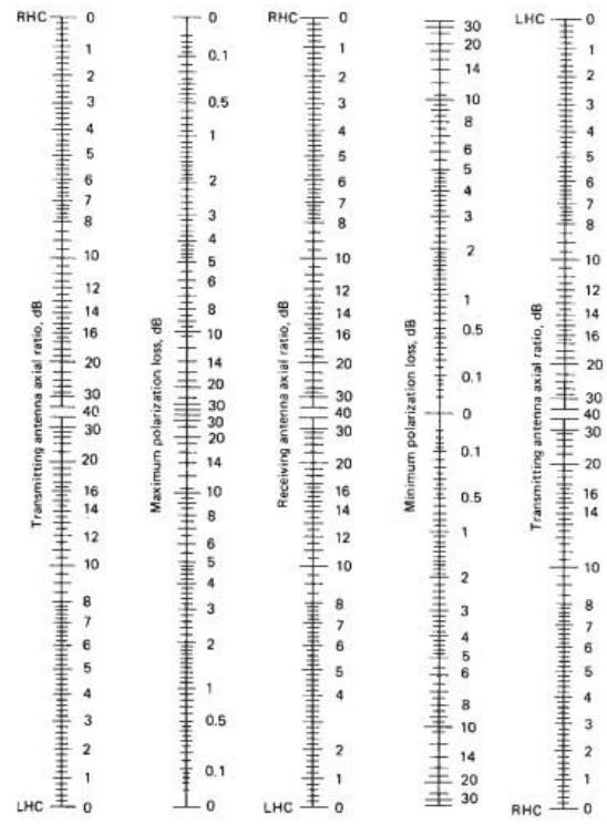Figure 3: Maximum and Minimum Polarization Loss given the Axial Ratio [37] A linear polarized wave is an elliptically polarized wave with an infinite axial ratio of infinity. For a linear polarization, the Eq. (28) is simplified to $$ X (d B) = 1 0 \log (\cos^ {2} (\theta) \tag {30} $$ In backscatter communication systems, we can define two polarization mismatches $X_{f}$ and $X_{b}$ that represent the forward and backward links, respectively. Polarization mismatch calculation $X_{f}$ and $X_{b}$ Let us consider three cases of antenna polarization for forward and backward links: - Case 1: LoRa transmitter, the tag and LoRa receiver antennas are all linearly polarized. - Case 2: LoRa transmitter and LoRa receiver antennas are right-hand circularly polarized, and the tag antenna is linearly polarized. - Case 3: LoRa transmitter, tag, and LoRa receiver antenna are all left-hand circularly polarized. Table 4 presents some values of the forward and backward polarization mismatch $X_{f}$ and $X_{b}$ given $\theta$ values computed using the assumption in case 1. In case 2, a linearly polarized tag antenna is trying to receive a circularly polarized wave from the LoRa transmitter which can be seen as two orthogonal linearly polarized waves with one in phase; therefore, the linearly polarized tag antenna will simply pick up the in-phase component of the circularly polarized wave from the LoRa transmitter, resulting in a forward polarization mismatch value $X_{f} = 0.5$. Similarly, the linearly polarized Table 4: Polarization Mismatch $X_{f}$ and $X_{b}$ Values Given $\theta$ for Case 1 <table><tr><td>Scenario</td><td>θf</td><td>θb</td><td>Xf</td><td>Xb</td></tr><tr><td>Scenario 1</td><td>0°</td><td>0°</td><td>1</td><td>1</td></tr><tr><td>Scenario 2</td><td>90°</td><td>90°</td><td>0</td><td>0</td></tr><tr><td>Scenario 3</td><td>24°</td><td>81°</td><td>0,83</td><td>0,02</td></tr><tr><td>Scenario 4</td><td>36°</td><td>59°</td><td>0,65</td><td>0,26</td></tr><tr><td>Scenario 5</td><td>63°</td><td>15°</td><td>0,20</td><td>0,93</td></tr><tr><td>Scenario 6</td><td>6°</td><td>11°</td><td>0,99</td><td>0,96</td></tr></table> receiver antenna will pick up the in-phase component of the circularly polarized wave from the tag, resulting in a backward polarization mismatch $X_{b}$ of 0.5. In case 3, we assume that all antennas are right-hand circularly polarized (RHCP). Similarly, Table 5 presents some values of the polarization mismatch for forward and backward links using the monograph in Figure 3, given the axial ratio in dB. Table 5: Polarization Mismatch $X_{f}$ And $X_{b}$ Values Calculated from Monograph in Figure 3 Given Axial Ratio Values for Case 3 <table><tr><td>Scenarios</td><td>\(A_{R_{TX}} \) dB</td><td>\(A_{R_{tag}} \) dB</td><td>\(A_{R_{RX}} \) dB</td><td>\(X_{f} \) dB</td><td>\(X_{b} \) dB</td></tr><tr><td>Scenario 1</td><td>0</td><td>0</td><td>0</td><td>0</td><td>0</td></tr><tr><td>Scenario 2</td><td>2.4</td><td>1.5</td><td>3</td><td>0.02</td><td>0</td></tr><tr><td>Scenario 3</td><td>5</td><td>2</td><td>0.8</td><td>0.1</td><td>0,02</td></tr><tr><td>Scenario 4</td><td>10</td><td>0.1</td><td>4</td><td>1</td><td>0,26</td></tr><tr><td>Scenario 5</td><td>7</td><td>2</td><td>5</td><td>0,3</td><td>0,93</td></tr></table> ## iii. Path Blockage Path blockage B represents the loss in the link budget that occurs when an obstruction, such as buildings, trees, ridges, bridges, vegetation, cliffs, etc., blocks the signal propagation path. The obstruction causes a non-line-of-sight (NLOS) between the transmitting and the receiving antennas. In [38], a frequency-dependent NLOS equation is defined to characterize the NLOS path loss as given as below. $$ PL^{NLOS} = 36.85 + 30 \log_{10}(d) + 18.9 \log_{10}(Fc) + \chi_{a}, $$ where $F_{c}$ is in GHz, $d$ is the distance between transmitter and receiver in meters, and $\chi_{a}$ is the shadowing component modelled according to a lognormal random variable with standard deviation $\sigma = 4dB$ [39] We calculate the values of the forward and backward path blockages $B_{f}$ and $B_{b}$ using Eq. (31). Since the carrier frequency is the same for the forward and backward links, and assuming the same value of the standard deviation $\sigma = 4dB$ for both links, the blockage loss values $B_{f}$ and $B_{b}$ will only depend on the transmitter-to-tag and tag-to-receiver distance and are given as: $$ B _ {f} = 3 6. 8 5 + 3 0 \log_ {1 0} \left(d _ {1}\right) + 1 8. 9 \log_ {1 0} \left(F _ {C}\right) + \chi_ {a}, \tag {32} $$ The Table 6 presents some values of path blockage computed at distances $d$ in the 915 MHz ISM band. Table 6: Path Blokage for Given Distances at 915 MHz ISM BAND <table><tr><td>Distance in (m)</td><td>Path blockage in (dB)</td></tr><tr><td>1</td><td>40.12</td></tr><tr><td>10</td><td>70.12</td></tr><tr><td>50</td><td>91.09</td></tr><tr><td>100</td><td>100.12</td></tr><tr><td>1000</td><td>130.12</td></tr><tr><td>10000</td><td>160.12</td></tr></table> The tag-to-receiver distance defined in Eq. (15) can be modified to account for the effect of path blockage on forward and backward links. First, let us express the Eq. (32) and (33) in linear form as follows. $$ B_{f} = 6487 \chi_{a} d_{1}^{3} $$ $$ B_{b} = 6487 \chi_{a} d_{2}^{3} $$ Replacing Eq. (34) and (35) in (15) will result in a tag-to receiver distance $d_{2}$ as- $$ d _ {2} ^ {N L O S} = \left. \frac {P _ {T} . G _ {T} . G _ {R} . G _ {t} ^ {2} . M . X _ {f} . X _ {b} . M . 2 ^ {S F}}{4 2 . 1 0 ^ {6} . S N R _ {0} . N F . K T . B W . \chi_ {a} ^ {2} . \theta . F _ {\beta}} (\frac {\lambda}{4 \pi}) ^ {4}\right) ^ {\frac {1}{3 n}} \frac {1}{d _ {1}} \tag {36} $$ ## iv. Fade Margin The fade margin results in interference from scattered waves that are caused by objects surrounding the environment of the tag. It is a function of the position of the RF tag, even in line-of-sight [27] and results in a variation of the backscattered signal and is known as small-scale fading [27]. Its value is calculated using the outage probability. The fade margin is defined as [27]: $$ F = 10 \log_{10} \left\{ \frac{F_{R}^{-1} (\text{outage probability})^{2}}{P_{av}} \right\} $$ Where, $P_{av}$ is the average channel power, and $F_{R}^{-1}$ is the cumulative distribution function of the received envelope. In this thesis, we assume a deployment in an agriculture application where there are few objects that can produce interference; therefore, the outage probability can be chosen as small. From [27], for an outage probability of 0.005 and a gain of 3dB, the calculated fade margin for a dislocated backscatter link was 26 dB. ## v. Tag on object gain The on-object antenna gain accounts for the losses when the RF tag is close to or attached to an object [27]. The value of $\theta$ depends on the properties of the material, the geometry of the object, the frequency, and the type of antenna. In [40], the values of $\theta$ for different materials have been measured using simulation. Table 7 shows some values of $\theta$ for various materials measured at 915MHZ [27, 40]. In this work, we assume the tag to be attached to a cardboard sheet. Table 7: On-Objet Antenna Gain Penalties for Various Material Measured at 915 mhz in Db [40] <table><tr><td>Material</td><td>θ (in dB)</td></tr><tr><td>Aluminum</td><td>10.4</td></tr><tr><td>De-lonized water</td><td>5.8</td></tr><tr><td>Acrylic Slab</td><td>1.1</td></tr><tr><td>Cardboard Sheet</td><td>0.9</td></tr></table> ### d) Concurrent transmission in LoRa backscatter and interference effects It has been shown that different tag signals can be decoded at the receiver, enabling concurrent transmission using the LoRa signal as excitation. Such receiver designs are commonly used in Internet of Things (IoT) applications where different sensors need to be deployed to cover the entire monitoring area. In [41] a LoRa backscatter configuration based on concurrent transmission was proposed for automatic irrigation monitoring where all sensor nodes transmit their data to a LoRa backscatter receiver. However, in such an implementation, some key challenges have to be addressed. Note that interfering signals contribute to the receiver noise power and hence reduce the SNR which affects the receiver performance and decreases the range. The key challenge while designing such receiver consists in removing the effect of interferences generated by the excitation signal (strong in-band interference) and the one from neighboring tags (inter-tag interference). These challenges have been addressed in [15, 42]. In [15], the inter-tag interference is addressed by using a hamming window that smoothly reduces signal amplitude toward zero from the centre to the edges. [15] also adds additional empty bins between two allocated bins to deal with the frequency and time offset caused by the difference in ToF (Time of Flight) between the tag and receiver. A similar technique is used in [42] to combat the time synchronization effect. Additionally, [42] uses a power-aware cyclic shift technique where lower SNR devices use a much different cyclic shift than higher SNR devices. On the basis of these observations, we extend our model to account for the effect of interference. Let us denote $I$ as the combined power of interfering signals that represents the total signal loss due to the interference. The value of $I$ depends on the receiver interference removal capability and on the combined received signal power from neighboring tags and transmitter (direct path) at the receiver location. Figure 4 illustrates a concurrent LoRa backscatter link. $d_{i11}$ and $d_{i12}$ are the forward and backward links separation distance for interfering tag 1, $d_{i21}$ and $d_{i22}$ are the forward and backward links separation distance for interfering tag 2, and $d_r$ is the distance between the LoRa transmitter and receiver. $P^{d_r}$ is the power received through the direct path (between the transmitter and the receiver). It is better for the receiver to eliminate interference and lower the value of $I$. Note that the interferences are non-coherent, i.e. they are not all at the same frequency and locked in phase. Therefore, the total interference power can be written as: $$ I = P _ {r} ^ {d} + \sum_ {i = 1} ^ {N} P _ {r i} ^ {t a g} \tag {38} $$ Where, $P_{r}^{d}, P_{ri}^{tag}$ are the received powers from the direct path (from the transmitter to the receiver) and the received power from the N neighboring tag (i.e. the interfering tags), respectively. Now, we define the signal-to-interference-plus-noise (SINR) as: $$ SINR = \frac{P_r}{P_n + I} $$ Where $P_{n}$ is the noise power. Note that the receiver sensitivity is inversely proportional to the level of interference. Using Eq. (9), the extended model accounting for the effect of interference of the achieved tagto-receiver distance for free space, LOS realistic, and NLOS realistic scenarios are given in Eq. 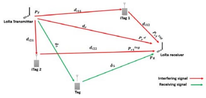(40), (41), and (42), respectively, as:  Figure 4: Concurrent Transmission Link Illustration $$ \begin{array}{l} d _ {2} ^ {F S} = \left(\frac{P _ {T} . G _ {T} . G _ {R} . G _ {t} ^ {2} . M . 2 ^ {S F}}{S N R _ {0} . (N F . K . T . B W + P _ {r} ^ {d} + \sum_ {i = 1} ^ {N} P _ {r i} ^ {\text{tag}})} (\frac{\lambda}{4 \pi}) ^ {4}\right) ^ {\frac{1}{n}} \frac{1}{d _ {1}} (40) \\d _ {2} ^ {L O S} = \left(\frac{P _ {T} . G _ {T} . G _ {R} . G _ {t} ^ {2} . X _ {f} . X _ {b} . M . 2 ^ {S F}}{S N R _ {0} . (N F . K . T . B W + P _ {r} ^ {d} + \sum_ {i = 1} ^ {N} P _ {r i} ^ {t a g}) . \theta . F _ {\beta}} \left(\frac{\lambda}{4 \pi}\right) ^ {4}\right) (41) \\\end{array} $$ The received power from the direct path $P_r^d$ and neighboring tags $P_{ri}^{tag}$ can be measured or computed using Eq. (43) and [44], respectively. $$ P _ {d} = P _ {T} G _ {T} G _ {R} \frac {\lambda^ {2}}{4 \pi} \frac {1}{d ^ {n}} \tag {42} $$ $$ P _ {r i} ^ {\text{tag}} = \frac{P _ {T} G _ {T} G _ {R} G _ {\text{tag} , i} ^ {2} X _ {f} X _ {b} M}{B _ {f} B _ {b} \theta F _ {\beta}} \left(\frac{\lambda}{4 \pi}\right) ^ {4} \left(\frac{1}{i d _ {i 1} i d _ {i 2}}\right) ^ {n} \tag{43} $$ ## IV. RESULTS AND DISCUSSION In this section, we evaluate our derived models in different scenarios. First, we evaluate the communication range of LoRa backscatter technology between a tag node and a receiver in free space propagation. We examine the effect of LoRa transmission parameters on the tag-to-receiver distance. In this paper, for a better illustration, we consider an application scenario in which the LoRa backscatter system is deployed to monitor an irrigation field as presented in Figure 13a. However, the model can be adapted for other types of application in both outdoor and indoor environments simply by changing some parameter values. We assume that the LoRa signal source will be generated by the LoRa radio chip SX1272. LoRa chip SX1272 uses a spreading factor that varies from 6 to 12 and operates in the frequency range of 860 to 1020 MHz [43]. We set the transmission frequency at 915 MHz and the transmit power at 20 dBm, which is the maximum allowed value in most regions. The LoRa provides three main transmission bandwidths: 125 KHZ, 250 KHZ, and 500 KHZ. We use the SX1308P915G LoRa gateway as the receiver which operates in the 915 MHZ band [44]. We fix the receiver noise figure at 6 dB and the minimum signal-to-noise ratio $(SNR_0)$ at 15 dB. Second, we evaluate the tag-to-receiver distance in a realistic scenario where additional losses are considered in the link budget in both the LOS and the NLOS scenarios. The modulation factor $M$ is equal to 0.5 for the BPSK, as given in Table 2. We also assumed a linear polarization for the transmitter, tag, and receiver antennas with an angle between the polarization vector of $36^{\circ}$ and $59^{\circ}$, resulting in a forward and backward polarization mismatch of 0.65 and 0.26 dB, respectively. We consider a tag attached to a cardboard Sheet which correspond to an tag-on-object gain penalty of 0.9dB. The fade margin is chosen to be 26dB as mentioned above. The path blockage effect is taken into account in the NLOS scenario and computed by Eq. (36). Moreover, the impacts of the above-mentioned parameters on the tag-to-receiver distance are also analyzed. Third, we extend our model to account for both in-band strong interference and that generated by concurrent tag transmission. In concurrent transmission, a single receiver receives several tags signal, increasing the interference noise power and the receiver complexity, as detailed in Section 3.4. The effect of the interfering tag is also analyzed in this section. The simulation parameters are summarized in Table 8 un-less otherwise stated. ### a) In Free Space Propagation We place the signal source at a fixed location, move the tag to different locations from the transmitter, and calculate the distance between the tag and the receiver. Figure 5 shows the com $$ d_{2}^{NLO S} = \left(\frac{P_{T}.G_{T}.G_{R}.G_{t}^{2}.X_{f}.X_{b}.M.2^{S F}}{42.10^{6}.S N R_{0}.(N F .K .T .B W + P_{r}^{d} + \sum_{i = 1}^{N} P_{r i}^{\text{tag}}) .\chi_{a}^{2} .\theta .F_{\beta}} \left(\frac{\lambda}{4 \pi}\right)^{4}\right)^{\frac{1}{3 n}} \frac{1}{d_{1}} \tag{42} $$ Table 8: Simulation Parameters <table><tr><td>Parameters</td><td>Values</td></tr><tr><td>Fc(MHz)</td><td>915</td></tr><tr><td>PT(dBm)</td><td>20</td></tr><tr><td>GT,GR(dBi)</td><td>2.4</td></tr><tr><td>Gt(dBi)</td><td>2.1</td></tr><tr><td>BW(KHz)</td><td>125</td></tr><tr><td>SNR0(dB)</td><td>15</td></tr><tr><td>SF</td><td>7</td></tr><tr><td>Path loss exponent n</td><td>3 for realistic case for free space case</td></tr><tr><td>M</td><td>0.5</td></tr><tr><td>Fβ(dB)</td><td>26</td></tr><tr><td>Xf</td><td>0.26</td></tr><tr><td>Xb</td><td>0.65</td></tr><tr><td>θ(dB)</td><td>0.9</td></tr><tr><td>NF(dB)</td><td>6</td></tr></table> munication range achieved between the RF tag and the LoRa receiver (distance d2) in free-space propagation using Eq. (11). When the Rf tag is in the vicinity of the transmitter (distance less than 1m), the receiver can be placed as far as $6.8\mathrm{km}$. This distance decreases as the transmitter-to-tag distance increases. For example, when the tag is placed 10m from the signal source, the receiver can be placed as far as 700m. At 60m from the transmitter, this distance drops to only about 114m. The midpoint between the LoRa transmitter and the receiver is measured at a distance $\mathrm{d}1 = \mathrm{d}2 = 88\mathrm{m}$, which translates to a total distance of 176m between the RF source and the receiver. Note that the maximum communication range of LoRa backscatter technology depends also on tag sensitivity; i.e. the maximum distance at which an RF tag can detect the transmitted signal, limiting its applications range. The higher sensitivity circuit can be used on the tag to increase the detection range to hundreds of meters [15, 45]. ## i. Effect of LoRa Parameters In this subsection, we analyze the effect of LoRa parameters, such as the spreading factor, bandwidth, and transmit power, on the LoRa backscatter range. LoRa uses different spreading factors. Now, we will increase the value of SF from 7 to 12 and visualize its impact on the communication range. As shown in Figure 6, the communication range increases with increasing SF value. For example, for a distance d1 of $20\mathrm{m}$, the receiver can be placed as far as $7.7\mathrm{km}$, $2.7\mathrm{km}$, and $1.3\mathrm{km}$ using SF values of 12, 9, and 7, respectively. By changing the spreading factor from 7 to 12 for a tag-to-source distance of $20\mathrm{m}$, we can improve the communication range by 6.4 km. 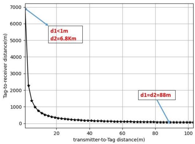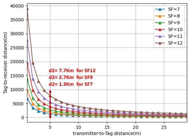However, for the LoRa communication system, higher throughput is achieved for small values of the spreading fac   Figure 5: Tag-To-Receiver Distance for Free Space Model as a Function of Transmitter-to-tag Distance (D1) tor [18]. Hence, there is a trade-off between throughput and range. For low data-rate applications such as automatic irrigation [41, 46], animal tracking [47], and forest fire detection, small values throughput can be tolerable; since the sensor node needs to transmit only a few bits of data. Similarly, we vary the transmit power from 7 dBm to 30 dBm and evaluate its impact on the tag-to-receiver distance. In Figure 7, it can be seen that the communication range varies with transmit power. Higher transmit power leads to a longer communication range. For example, when we move the RF tag 5m away from the transmitter, the receiver can be placed as far as 0.3 Km, 0.7 Km, 1.3 Km, and 4.3 Km for transmit power of 7 dBm, 14 dBm, 20 dBm, and 30 dB, respectively. In other words, an increase of 6dB in transmit power improves the communication range by $47\%$. 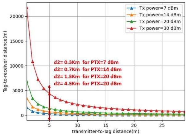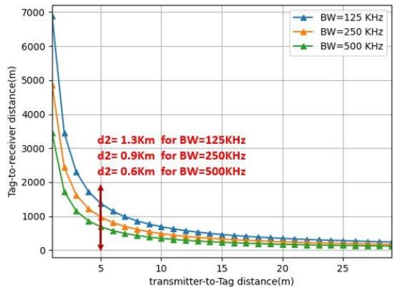Note that a higher transmit power trans-  Figure 6: Tag-to-Receiver Distance for Free Space Model as a Function of Transmitter-to-Tag Distance (D1) for Different SF  Figure 7: Tag-to-Receiver Transmission Range for Free Space Model as a Function of Transmitter-to-Tag Distance (D1) Figure 8: Tag-To-Receiver Transmission Range in Free Space Model as a Function of Transmitter-to-Tag Distance (D1) for Different Lora Transmission Bandwidths  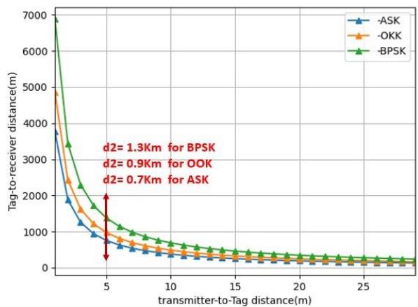Figure 9: Tag-To-Receiver Ranges in Free Space Model for Different Modulation Schemes lates into higher energy consumption. In addition, in backscatter communication systems, the direct signal received from the transmitter creates interference, which limits the detection of the weak backscatter signal from the tag at the receiver. 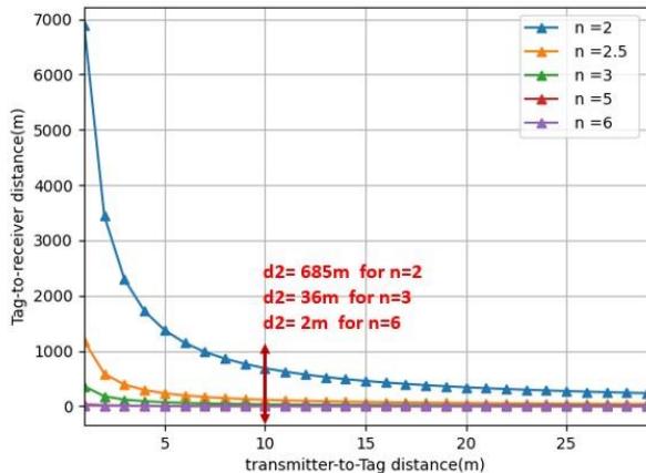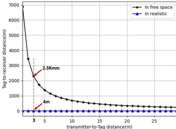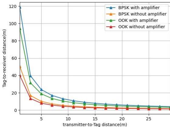In the literature, direct interference cancellation techniques have been  Figure 10: Tag-to-Receiver Transmission Range as a Function of Transmitter-to Tag Distance (D1) Different Path Loss Exponent  Figure 11: Tag-To-Receiver Distance Comparison Between Free Space and Realistic Model Corrected Version Under Same Antenna Gain ( $G_{T} = G_{R} = G_{t} = 1$ )  Figure 12: Reflection Amplifier Effect on tag-to-Receiver Range for BPSK and OOK Modulation Scheme proposed to mitigate the strong interference effect and improve the SNR [16, 17, 23]. The variation in bandwidth as a function of distance is shown in Figure 8. 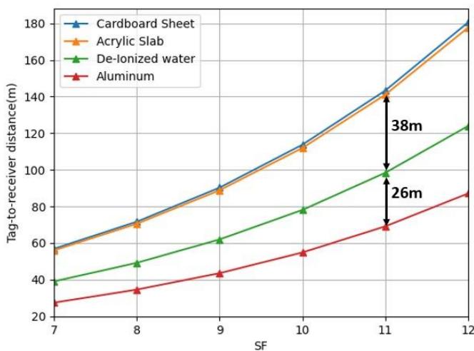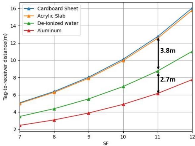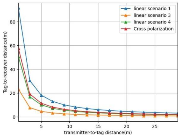We observe that the distance  (a) $d1 = 1m$  (b) $d / 1 = 10m$  (c) $d1 = 50\mathrm{m}$  (d) $d / 1 = 100\mathrm{m}$  Figure 13: Tag-to-Receiver Distance as a Function of SF for Different on Object Gain Penalty and Fixed Distance D1 Figure 14: Tag-to-Receiver Range in Free Space Model for Different Transmitter, Tag, and Receiver Antennas Polarization decreases with increasing LoRa bandwidth. For example, the communication range drops from $1.3\mathrm{Km}$ to $0.6\mathrm{Km}$ by increasing the bandwidth from $125\mathrm{KHz}$ to $500\mathrm{KHz}$. The communication range of LoRa backscatter systems can also vary parameters, such as the modulator factor and the path loss exponent. ## iii. Effects of Modulation Factor on LoRa Backscatter Range ii. Effects of Environment on Lora Backscatter Range - The path loss exponent describes the nature of the propagation environment. Figure 10 shows its impacts on the communication range. For a source-to-tag distance of $10\mathrm{m}$, the communication range is up to $685\mathrm{m}$ using a path loss value of 2, which corresponds to the case of free space propagation. As the path loss exponent increases, the range decreases, as shown in the figure. For the rest of this work, we assume a path loss value of 3, which is the worst case in the outdoor environment. In backscatter communication systems, the communication range is depends on tag scattering efficiency, which is also referred to as the modulator factor $M$. The tag modulation factor $M$ depends on the modulation scheme used to backscatter the tag data to the receiver, as discussed in Section 3.3.1. We vary the value of $M$ according to different modulation schemes as shown in Table 2 and compute the communication range for each value of $M$. In Figure 9, it can be seen that the BPSK achieves the highest communication range compared to ASK and OOK. However, the ASK scheme is more simple to implement than the BPSK. When the tag is placed at $5\mathrm{m}$, the BPSK scheme can reach the $1.3\mathrm{km}$ communication range while only $0.7\mathrm{km}$ is possible using ASK. ### b) Realistic Scenario In this subsection, we will evaluate the LoRa backscatter range in a realistic scenario in both LOS and NLOS. In a realistic scenario, different parameters affect the communication range between the RF tag and the LoRa receiver, as detailed in Section 3.2. ## i. In Line-of-Sight We compare the communication range of the free space model and the realistic scenario model in LOS (path blockage ignored) using Eq. (11) and (15). In Figure 11, it can be seen that the achieved range in the realistic case is much lower than that of the free space case. For example, for a source-to-tag distance of $3\mathrm{m}$, a communication range of $2.3\mathrm{km}$ is achieved, compared to only $4\mathrm{m}$ for the realistic LOS scenario using unit antenna gain for both transmitter, the tag, and receiver. This difference becomes important as the tag is brought close to the transmitter. 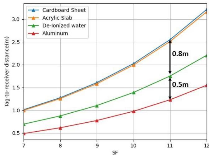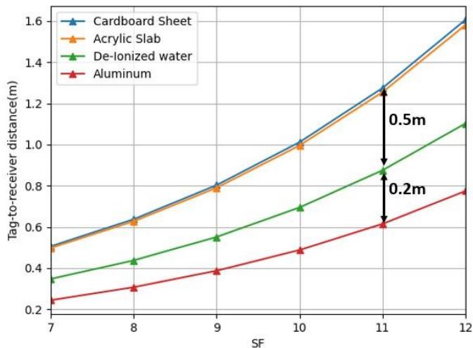To further improve the LoRa backscatter communication range, a reflection amplifier can be used [35]. To evaluate the effect of the reflection amplifier on the communication distance, we compare the range with and without the reflection amplifier in the realistic LOS scenario, as shown in Figure 12. We can observe an increase in the range when a reflection amplifier is used. Next, we evaluate the effect of tag-on-object gain in the communication range. As discussed in Section 3.3.5, different materials have different impacts on the performance of tag communication. Figure 13 shows the communication range as a function of the spreading factor for a tag attached to various materials. The cardboard sheet has the best performance, which is close to one obtained using an Acrylic slab. For a source-to tag distance of $1\mathrm{m}$, the communication range of $180\mathrm{m}$ for an SF value of 12 is achieved for a cardboard sheet compared to only $83\mathrm{m}$ with aluminum. Note also that the impact of the material becomes important as the SF values increase. However, as we increase the source-to-tag distance, the effect of the attached material becomes negligible as shown in Figure 13d. There was only a decrease of 0.7 between the cardboard sheet and the aluminum. Antenna polarization is another cause of signal attenuation and hence limits the communication range. Figure 14 shows the communication range achieved in different polarizations. It can be noticed that the linear polarization in Scenarios 1 has a better communication range (about $97\mathrm{m}$ ) compared to linear scenarios 3 and 4. This is due to the fact that, in the linear polarisation of Scenario 1, the polarization mismatches $X_{f}$ and $X_{f}b$ are maximal ( $X_{f} = X_{f}b = 1$ ). 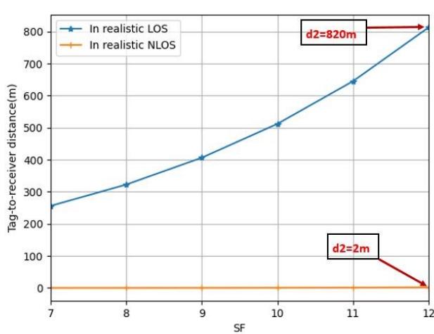### c) In NON Line-of-Sight (NLOS) In some applications, the LOS cannot be guaranteed, hence we must account for the effect of path blockage between the transmitter and tag antenna, and between tag and receiver antenna. We compare the maximum theoretical communication range of LoRa backscatter technology in both LOS and NLOS as shown in Figure 15. We set the value of M at 6.48 which is the maximum value in Table 3, and the transmit power at 30dBm. As can be seen from the figure, for a source-to-tag distance of 1m and an SF of 12, the receiver can be as far as 820m for LOS while only a range of 2m is possible in NLOS scenario. As the tag is moved away from the source, this distance drops to only 8.12m and 0.02m for LOS and NLOS, respectively. 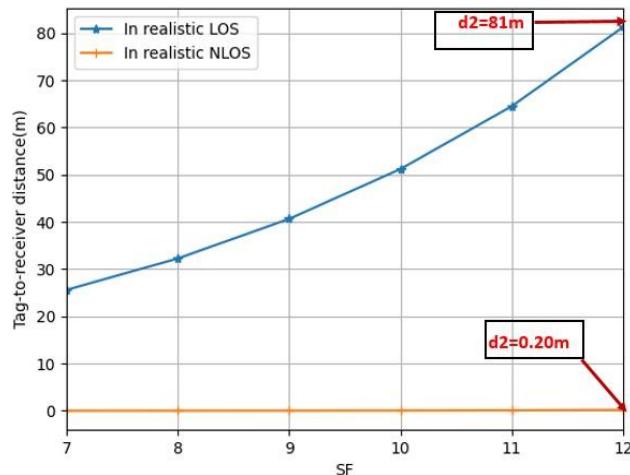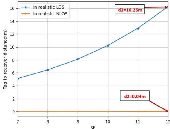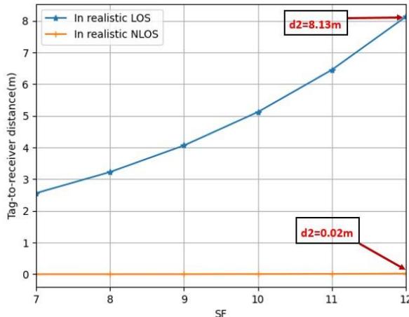This compromises the long-range wisdom of LoRa backscatter and  (a) $d1 = 1m$  (b) $d1 = 10\mathrm{m}$  (c) $d^{\prime}1 = 50m$  (d) $d1 = 100\mathrm{m}$ Figure 15: Maximum Tag-to-Receiver Range Comparison between LOS and NLOS Model for Fixed Distance D1 with A Maximum Transmit Power $P_{T} = 30$ dbm hence limits the range of its application deployment where there is no LOS between transmitter, tag, and receiver antennas. 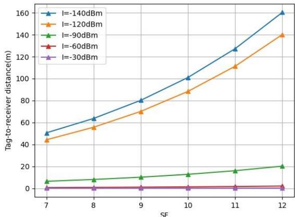### d) Concurrent Transmission and Interference Effect The performance of LoRa backscatter system degrades in the presence of strong interference from the transmitter and the inter-tag interference from the neighboring tags in concurrent transmission as discussed in Section 3.4. The effect of interference on the receiving distance depends on the signal level of the interfering signal at the receiver location, which also depends on the separation distance between the transmitter and the tag. First, we consider a LoRa backscatter system in which only one tag can transmit data to the receiver at a given instant $t$. Therefore, interferences from neighboring tags are ignored. We vary the values of direct interference power $P_{r}^{d}$ from -140 dBm to -30 dBm. Figure 16 shows the distance achieved between the tag and the receiver for different values of direct interference power in the LOS scenario. It can be noticed that when the level of interference signal power is low, for example -140dBm, the receiver can decode the backscatter signal at a distance of about 160m from the tag for a source-to-tag distance of 1m and a SF value of 12. As the level of interference signal increases, the receiver sensitivity decreases, and the distance achieved drops to 140m, 20m, and 2m for interference power of -120 dBm, -90 dBm, -60 dBm, respectively. For interference signal levels higher than -30dBm, the receiver cannot work anymore. One way to mitigate the interference effect is to increase the transmit power. Several other interference cancellations for LoRa backscatter systems have been proposed in the literature [15, 16, 23]. Another source of interference in LoRa backscatter systems is the inter-tag-interference. The signal received from the neighboring tags is very weak. However, the LoRa receiver has a high sensitivity, hence a receiver can receive both the desired tag signal and interference from neighboring tags. We fix the value of direct interference power to -120 dBm. We assume that all tags have received power at the receiver location of - 140 dBm and evaluate the effect of the number of neighboring tags on the tag-to-receiver distance. The range decreases as the number of interfering tags increases, as shown in Figure 17. Note that in practice, the received powers from both the neighboring tag and the transmitter are randomly distributed and vary depending on the channel condition. ### e) Evaluation of Our Model To evaluate the accuracy of our model, we will run different simulations using the same experiment setup and under the same scenario as the state-of-the art LoRa backscatter systems. The simulation parameters are shown in Table 9. It can be seen that the range achieved in our model is close to that obtained in practice for works PLoRa [18], $P^2$ LoRa [15], Aloba [14]. PLoRa uses frequency shift keying to encode tag information. The range achieved using our model is significantly higher than the one obtained in PLoRa (about $55\%$ ). This is due to the poor interference cancellation in PLoRa. 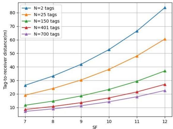Additionally, the PLoRa tag uses packet detection with a limited range  Figure 16: Direct Interference Effect on Lora Backscatter Communication Range  Figure 17: Number of Interfering Tag Effects on Lora Backscatter Communication Range for Identical Neighboring Tag Power of -120 dbm and a Fixed Direct Interference Power of -110 dbm Table 9: Comparison of Our Range Model with Existing Lora Backscatter Prototypes Achieved Range in The Literature. Note That the Reported Ranges are Measured in A Line-Of-Sight (LOS) Scenario <table><tr><td>Parameters</td><td>PLoRa</td><td>P2LoRa</td><td>ALOBA</td><td>LoRa backscatter</td></tr><tr><td>Modulation type</td><td>FSK</td><td>FSK</td><td>OOK</td><td>CSS</td></tr><tr><td>Tx power</td><td>21dBm</td><td>30 dBm</td><td>20dBm</td><td>30dBm</td></tr><tr><td>Tx gain</td><td>2dBi</td><td>4dBi</td><td>3 dBi</td><td>6 dBi</td></tr><tr><td>Rx gain</td><td>2dBi</td><td>4dBi</td><td>3 dBi</td><td>6 dBi</td></tr><tr><td>tag gain</td><td>2dBi</td><td>4 dBi</td><td>3 dBi</td><td>2 dBi</td></tr><tr><td>SF</td><td>8</td><td>12</td><td>12</td><td>12</td></tr><tr><td>BW</td><td>500KHz</td><td>31.25 kHz</td><td>125KHz</td><td>31.25 kHz</td></tr><tr><td>Fc</td><td>915 MHz</td><td>433 MHz</td><td>902.5MHz</td><td>915 MHz</td></tr><tr><td>d1</td><td>20 cm</td><td>1m</td><td>1m</td><td>5 m</td></tr><tr><td>Range</td><td>1.1Km</td><td>2.2Km</td><td>250 m</td><td>2.8Km</td></tr><tr><td>Our model</td><td>2Km</td><td>2.5Km</td><td>206m</td><td>188m</td></tr></table> of 50m which limits the overall range of the system. Moreover, the frequency-shifting operation in backscatter communication introduces mirror copies of the backscatter signal and spreads the energy in double sidebands which significantly degrades the SNR, hence limiting the communication range. Aloba[14] range is similar to one obtained using our model. The short range of Aloba is due to the OOK modulation which sacrifices the range for better throughput. Additionally, Aloba checks the amplitude and phase characteristics of the signal in the time domain, which results in a limited accumulated energy and hence a limited range. For $P^2$ LoRa[15], the theoretical range computed using our model is slightly higher than the one obtained during their experiment about $12\%$, and this may be due to the effect of the environment and losses due to the surrounding materials. Notice that $P^2$ LoRa achieved better communication range over both PLoRa and Aloba, this can be explained by the fact that they combine the energy in double sidebands to enhance the SNR. On the other hand, for LoRa backscatter [16] the achieved range during their experiment is about $2.8$ Km while using our method, this range is only $188$ m. To understand this, note that [16] synthesizes the LoRa compatible packet at the tag, while the state-of-the-art work mentioned above simply backscatters the ambient LoRa signal. This means that our model is not compatible with the LoRa backscatter system, where the tag generates a LoRa signal. Therefore, a more extensive model is required to cover all possible LoRa backscatter systems, and this is left for future research work. ## V. CONCLUSION In this work, we have developed a model to estimate the transmission range in LoRa backscatter communication. The developed model is based on both free space and a realistic LOS and NLOS propagation scenario. Throughout the simulation in Python, we analyzed the effect of different parameters that can affect transmission performance and discussed techniques to enhance link quality. We have also extended our model to account for the effect of interference from both the direct signal and the neighboring tags in concurrent transmission. We have also evaluated the accuracy of our model by comparing the range achieved using our model with state-of-the-art LoRa backscatter works. The developed model model is a useful tool for estimating coverage and deployment cost in real wireless sensor network applications. ### ACKNOWLEDGMENTS This work was funded by the National Natural Science Foundation of China under Grant No 61871174. #### REFERENCES RÉFERENCESREFERENCIAS 1. Shadi Al-Sarawi, Mohammed Anbar, Kamal Alieyan, and Mahmood Alzubaidi. Internet of things (iot) communication protocols: Review. In 2017 8th International Conference on Information Technology (ICIT), pages 685-690, 2017. 2. Adrian loan PETRARIU and Alexandru LAVRIC. Sigfox wireless communication enhancement for internet of things: A study. In 2021 12th International Symposium on Advanced Topics in Electrical Engineering (ATEE), pages 1-4, 2021. 3. Laura Joris, Franc,ois Dupont, Philippe Laurent, Pierre Bellier, Serguei Stoukatch, and Jean-Michel Redoute. An autonomous sigfox wireless sensor node for environmental monitoring. IEEE Sensors Letters, 3(7):01-04, 2019. 4. Kwon Nung Choi, Harini Kolamunna, Akila Uyanwatta, Kanchana Thilakarathna, Suranga Seneviratne, Ralph Holz, Mahbub Hassan, and Albert Y. Zomaya. Loradar: Lora sensor network monitoring through passive packet sniffing. SIGCOMM Comput. Commun. Rev., 50(4):10-24, oct 2020. 5. Jian-xiong Wang, Yang Liu, Zhi-bin Lei, Kang-heng Wu, Xiao-yu Zhao, Chao Feng, Hong-wei Liu, Xuehua Shuai, Zhong-min Tang, Li-yang Wu, Shao-yun Long, and Jia-rong Wu. Smart water lora IoT system. In Proceedings of the 2018 International Conference on Communication Engineering and Technology, ICCET '18, page 48-51, New York, NY, USA, 2018. Association for Computing Machinery. 6. Jin-Ping Niu and Geoffrey Ye Li. An overview on backscatter communications. Journal of Communications and Information Networks, 4(2):1-14, 2019. 7. Spyridon Nektarios Daskalakis, George Goussetis, Stylianos D. Assimonis, Manos M. Tentzeris, and Apostolos Georgiadis. A uw backscattermorse-leaf sensor for low-power agricultural wireless sensor networks. IEEE Sensors Journal, 18(19):7889-7898, 2018. 8. Eleftherios Kampianakis, John Kimionis, Konstantinos Tountas, Chris Konstantopoulos, Eftichios Koutroulis, and Aggelos Bletsas. Backscatter sensor network for extended ranges and - low cost with frequency modulators: Application on wireless humidity sensing. In SENSORS, 2013 IEEE, pages 1-4, 2013. 9. Vincent Liu, Aaron N. Parks, Vamsi Talla, Shyamnath Gollakota, David Wetherall, and Joshua R. Smith. Ambient backscatter: wireless communication out of thin air. Proceedings of the ACM SIGCOMM 2013 conference on SIGCOMM, 2013. 10. Huynh Nguyen, Hoang Dinh Thai, Xiao Lu, Dusit Niyato, Ping Wang, and Dong In Kim. Ambient backscatter communications: A contemporary survey. IEEE Communications Surveys & Tutorials, PP, 12 2017. 11. Dinesh Bharadia, Kiran Raj Joshi, Manikanta Kotaru, and Sachin Katti. Backfi: High throughput wifi backscatter. Proceedings of the 2015 ACM Conference on Special Interest Group on Data Communication, 2015. 12. Anran Wang, Vikram Iyer, Vamsi Talla, Joshua R. Smith, and Shyamnath Gollakota. FM backscatter: Enabling connected cities and smart fabrics. In 14th USENIX Symposium on Networked Systems Design and Implementation (NSDI '17), pages 243-258, Boston, MA, March 2017. USENIX Association. 13. Ritayan Biswas, Joonas Sae, and Jukka Lempiainen. Evaluation of maxi-mum range for backscattering communications utilising ambient fm radio signals. In 2022 International Balkan Conference on Communications and Networking (BalkanCom), pages 142-146, 2022. 14. Xiuzhen Guo, Longfei Shangguan, Yuan He, Jia Zhang, Haotian Jiang, Awais Siddiqi, and Yu Liu. Efficient ambient lora backscatter with on-off keying modulation. IEEE/ACM Transactions on Networking, PP:1-14, 11 2021. 15. Jinyan Jiang, Zhenqiang Xu, Fan Dang, and Jiliang Wang. Long-range ambient lora backscatter with parallel decoding. Proceedings of the 27th Annual International Conference on Mobile Computing and Networking, 2021. 16. Vamsi Talla, Mehrdad Hessar, Bryce Kellogg, Ali Najafi, Joshua R. Smith, and Shyamnath Gollakota. Lora backscatter: Enabling the vision of ubiquitous connectivity. Proc. ACM Interact. Mob. Wearable Ubiquitous Technol., 1(3), sep 2017. 17. Mehrdad Hessar, Ali Najafi, and Shyamnath Gollakota. NetScatter: Enabling Large-Scale backscatter networks. In 16th USENIX Symposium on Networked Systems Design and Implementation (NSDI '19), pages 271-284, Boston, MA, February 2019. USENIX Association. 18. Yao Peng, Longfei Shangguan, Yue Hu, Yujie Qian, Xianshang Lin, Xiaojiang Chen, Dingyi Fang, and Kyle Jamieson. Plora: a passive long-range data network from ambient lora transmissions. In SIGCOMM '18: ACM SIGCOMM 2018 Conference, pages 147-160, 08 2018. 19. Ganghui Lin, Ahmed Elzanaty, and Mohamed-Slim Alouini. Lora backscatter communications: Temporal, spectral, and error performance analysis. IEEE Internet of Things Journal, pages 1-1, 2023. 20. SIAKA KONATE, Changli Li, and Lizhong Xu. Theoretical evaluation of the performance of ambient lora backscatter communication. page 41, 06 2023. 21. Siaka Konate, Changli Li, and Lizhong Xu. Review on Iora backscatter technology. Future Generation Computer Systems, 167:107742, 2025. 22. Daniel Belo, Ricardo Correia, Yuan Ding, Spyridon Nektarios Daskalakis, George Goussetis, Apostolos Georgiadis, and Nuno Borges Carvalho. Iq impedance modulator front-end for low-power lora backscattering devices. IEEE Transactions on Microwave Theory and Techniques, 67(12):5307-5314, 2019. 23. Mohamad Katanbaf, Anthony Weinand, and Vamsi Talla. Simplifying backscatter deployment: Full-Duplex LoRa backscatter. In 18th USENIX Symposium on Networked Systems Design and Implementation (NSDI 21), pages 955-972. USENIX Association, April 2021. 24. Xiaoqing Tang, Guihui Xie, and Yongqiang Cui. Self-sustainable longrange backscattering communication using rf energy harvesting. IEEE Internet of Things Journal, 8(17):13737-13749, 2021. 25. H.T. Friis. A note on a simple transmission formula. Institute of Electrical and Electronics Engineers (IEEE), 35(5):254-256, May 1946. 26. Semtech sx1276 transceiver, 2020. https://www.semtech.fr/products/wirelessrf/lora-connect/sx1276. 27. Joshua D. Griffin and Gregory D. Durgin. Complete link budgets for backscatter-radio and rfid systems. IEEE Antennas and Propagation Magazine, 51, 2009. 28. J. T. Prothro and G. D. Durgin. Improved performance of a radio frequency identification tag antenna on a metal ground plane, 2007. 29. D. M. Dobkin. The RF in RFID: Passive UHF RFID in Practice. Australia: Elsevier, 2008. 30. J.-P. Curty, N. Joehl, C. Dehollain, and M.J. Declercq. Remotely powered addressable uhf rfid integrated system. IEEE Journal of Solid-State Circuits, 40(11):2193-2202, 2005. 31. Udo Karthaus and Martin Dipl.-Ing. Fischer. Fully integrated passive uhf rfid transponder ic with 16.7- $\mu$ w minimum rf input power. IEEE J. Solid State Circuits, 38:1602-1608, 2003. 32. John Kimionis, Aggelos Bletsas, and John N. Sahalos. Increased range bistatic scatter radio. IEEE Transactions on Communications, 62(3):1091-1104, 2014. 33. P. Chan and V. Fusco. Bi-static 5.8ghz rfid range enhancement using retrodirective techniques. In 2011 41st European Microwave Conference, pages 976-979, 2011. 34. Axel Strobel, Christian Carlowitz, Robert Wolf, Frank Ellinger, and Martin Vossiek. A millimeter-wave low-power active backscatter tag for fmcw radar systems. IEEE Transactions on Microwave Theory and Techniques, 61(5):1964-1972, 2013. 35. John Kimionis, Apostolos Georgiadis, Ana Collado, and Manos M. Tentzeris. Enhancement of rf tag backscatter efficiency with low-power reflection amplifiers. IEEE Transactions on Microwave Theory and Techniques, 62(12):3562-3571, 2014. 36. Rastislav Galuscak and Pavel Hazdra. Circular polarization and polarization losses. In in Proc. Du Bus, pages 8-23, 01 2006. 37. Thomas A. Milligan. Modern antenna design. John Wiley & Sons, Inc., Hoboken, New Jersey, 2005. 38. 3GPP. Study on evaluation methodology of new vehicle-to-everything (v2x) use cases for lte and nr (release 15), 2019. TR 37.885. 39. 3GPP. "study on lte-based v2x services (release 14), 2016. TR 36.885." 40. J. D. Griffin, G. D. Durgin, A. Haldi, and B. Kippelen. Rf tag antenna performance on various materials using radio link budgets. IEEE Antennas and Wireless Propagation Letters, 5:247-250, 2006. 41. Siaka Kionate, Changli Li, and Lizhong Xu. Lora backscatter automated irrigation approach: Reviewing and proposed system. In 2020 6th International Conference on Robotics and Artificial Intelligence, ICRAI 2020, page 205-213, New York, NY, USA, 2020. Association for Computing Machinery. 42. Mehrdad Hessar, Ali Najafi, and Shyamnath Gollakota. NetScatter: Enabling Large-Scale backscatter networks. In 16th USENIX Symposium on Networked Systems Design and Implementation (NSDI '19), pages 271-284, Boston, MA, February 2019. USENIX Association. 43. Semtech Sx1272 Datasheet. Low power long range transceiver, Jan. 2019. https://www-semtech.fr/ products/wireless-rf/lora-connect/sx1272. 44. Semtech Sx1308 Datasheet. Wireless & sensing products, June 2017. https://www.semtech.fr/products/wireless-rf/lora-core/sx1308p868gw. 45. Xiuzhen Guo, Longfei Shangguan, Yuan He, Nan Jing, Jiacheng Zhang, Haotian Jiang, and Yunhao Liu. Saiyan: Design and implementation of a low-power demodulator for LoRa backscatter systems. In 19th USENIX Symposium on Networked Systems Design and Implementation (NSDI 22), pages 437-451, Renton, WA, April 2022. Usenix Association. 46. S. R. Jino Ramson and D. Jackuline Moni. Applications of wireless sensor networks - a survey. In 2017 International Conference on Innovations in Electrical, Electronics, Instrumentation and Media Technology (ICEEIMT), pages 325-329, 2017. 47. Tanveer Baig z and Chandrasekar Shastry. Design of wsn model with ns2 for animal tracking and - monitoring. Procedia Computer Science, 218:2563-2574, 2023. International Conference on Machine Learning and Data Engineering.

Generating HTML Viewer...