Obtaining the Sinusoid for Working with Membrane Vibration from the Bessel Differential Equation

Obtaining the Sinusoid for Working with Membrane Vibration from the Bessel Differential Equation

Article Fingerprint

ReserarchID

TP971

Obtaining the Sinusoid for Working with Membrane Vibration from the Bessel Differential Equation Banner

AI TAKEAWAY

Connecting with the Eternal Ground
  • English
  • Afrikaans
  • Albanian
  • Amharic
  • Arabic
  • Armenian
  • Azerbaijani
  • Basque
  • Belarusian
  • Bengali
  • Bosnian
  • Bulgarian
  • Catalan
  • Cebuano
  • Chichewa
  • Chinese (Simplified)
  • Chinese (Traditional)
  • Corsican
  • Croatian
  • Czech
  • Danish
  • Dutch
  • Esperanto
  • Estonian
  • Filipino
  • Finnish
  • French
  • Frisian
  • Galician
  • Georgian
  • German
  • Greek
  • Gujarati
  • Haitian Creole
  • Hausa
  • Hawaiian
  • Hebrew
  • Hindi
  • Hmong
  • Hungarian
  • Icelandic
  • Igbo
  • Indonesian
  • Irish
  • Italian
  • Japanese
  • Javanese
  • Kannada
  • Kazakh
  • Khmer
  • Korean
  • Kurdish (Kurmanji)
  • Kyrgyz
  • Lao
  • Latin
  • Latvian
  • Lithuanian
  • Luxembourgish
  • Macedonian
  • Malagasy
  • Malay
  • Malayalam
  • Maltese
  • Maori
  • Marathi
  • Mongolian
  • Myanmar (Burmese)
  • Nepali
  • Norwegian
  • Pashto
  • Persian
  • Polish
  • Portuguese
  • Punjabi
  • Romanian
  • Russian
  • Samoan
  • Scots Gaelic
  • Serbian
  • Sesotho
  • Shona
  • Sindhi
  • Sinhala
  • Slovak
  • Slovenian
  • Somali
  • Spanish
  • Sundanese
  • Swahili
  • Swedish
  • Tajik
  • Tamil
  • Telugu
  • Thai
  • Turkish
  • Ukrainian
  • Urdu
  • Uzbek
  • Vietnamese
  • Welsh
  • Xhosa
  • Yiddish
  • Yoruba
  • Zulu
Font Type
Font Size
Font Size
Bedground

Abstract

To study membranes’ acoustic behavior there are several equations concerning their vibration and resonance which help us to understand better their physical properties. In the present paper we want to show the results of the Bessel sinusoid expressions when we change the values of their variables. Because the procedures to solve the Bessel equation are usually not shown in their entirety in books or the Internet this paper explains in detail each step to go from its differential expression to the sinusoid one.

I. INTRODUCTION

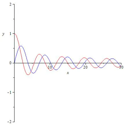
It is well known that the expression J 0 of Bessel equations is the graphic most widely published in Differential Equation textbooks. Every time we talk about the vibration of a circular membrane the graphics of Figure 1is always referred to. Mathematical software packages such as MapleTM always includes this curve in their libraries. If you hit once a circular membrane, it is easy to assume that the first undulation will have a higher amplitude than the following undulations which will decrease gradually as shown also in Figure 1.

T h e p l o t o f B e s s e l f u n c t i o n s J 0 a n d J 1 plot ( [ BesselJ ( 0 , x ) , BesselJ ( 1 , x ) ] , x = 0. . 3 0 , y = 2. . 2 , color = [ red , blue ] )
Figure 1: Plot of J0 and J1 of Bessel

In this work we proceed to find the Jv ( x ) functions of the first kind and order v to satisfy the second order differential equation of Bessel.

x 2 d 2 y ( x ) d x 2 + x d y ( x ) d x + ( x 2 v 2 ) y ( x ) = 0

To study acoustical radiation and vibration analysis one usually solves problems in cylindrical coordinates that are associated with Bessel functions of integer order. We can solve also spherical problems with half-integer order Bessel Function.

II. BESSEL FUNCTIONS

a) Differential Equation of Oder ν

Wefocus this work on Besselfunctions of the first kind of positive order and real arguments[1]for

x 2 y + x y + ( x 2 v 2 ) y = 0

Assuming

y = 0 c n x n + r

which leads to

Differentiating and substituting

y = c n ( n + r ) X n + r 1
y = c n ( n + r ) ( n + r 1 ) X n + r 2
x 2 y + x y + ( x 2 v 2 ) y = 0
x 2 c n ( n + r ) ( n + r 1 ) x n + r x 2
c n ( n + r ) ( n + r 1 ) x n + r
x 2 y + x y + ( x 2 v 2 ) y = 0
x c n ( n + r ) x n + r x 1
x 2 y + x y + ( x 2 v 2 ) y = 0
c n ( x 2 v 2 ) x n + r

Writing out the differential equation give us

n = 0 c n ( n + r ) ( n + r 1 ) x n + r + n = 0 c n ( n + r ) x n + r + n = 0 c n x n + r + 2 v 2 n = 0 c n x n + r
F o r n = 0
c 0 ( r ) ( r 1 ) x r + c 0 ( r 2 r ) x r + c 0 r x r + c 0 x r + 2 c 0 v 2 x r

Substituting this back to the differential equation gives

c 0 ( r 2 r + r v 2 ) x r + x r n = 1 c n [ ( n + r ) ( n + r 1 ) + ( n + r ) v 2 ] x n + x r n = 0 c n x n + 2
( n + r ) ( n + r 1 ) + ( n + r )
( n + r ) ( n + r + 1 ) = n 2 + 2 n r + r 2 n r
n 2 + 2 n r + r 2 n r + ( n + r )
n 2 + 2 n r + r 2
( n + r ) 2

Leading to

c 0 ( r 2 v 2 ) x r + x 2 n = 1 c n [ ( n + r ) 2 v 2 ] x n + x r n = 1 c n x n + 2 = 0

If r 1 = v

[ ( n + v ) 2 v 2 ] = n 2 + 2 n v + v 2 v 2
n ( n + 2 v )

giving

x v n = 1 c n n ( n + 2 v ) x n + x v n = 0 c n x n + 2
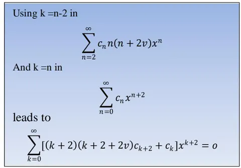
x v c 1 ( 1 + 2 v ) + n = 2 c n n ( n + 2 v ) x n + n = 0 c n x n + 2

Writing this out

x v c 1 ( 1 + 2 v ) + k = 0 [ ( k + 2 ) ( k + 2 + 2 v ) c k + 2 + c k ] x k + 2 = 0

So that

( 1 + 2 v ) = 0
( k + 2 ) ( k + 2 + 2 v ) c k + 2 + c k = 0

Or

c k + 2 = c k ( k + 2 ) ( k + 2 + 2 ν ) k = 0 , 1 , 2. .

c 1 = 0 in (1) leads toc 3 = c 5 = c 7 = = 0 so, for k = 0 , 2 , 4 . after making k + 2 = 2 n , n = 1 , 2, 3.. we will have that

c 2 n = c 2 n 2 2 n ( 2 n + 2 v )
c 2 n 2 2 2 n ( n + v )

The coefficients with even index are determined by the following formula:

c 2 = c 0 2 2 1 ( 1 + v )
c 4 = c 2 2 2 2 ( 2 + v ) = c 0 2 4 1 2 ( 1 + v ) ( 2 + v )
c 6 = c 4 2 2 3 ( 3 + v ) = c 0 2 6 1 2 3 ( 1 + v ) ( 2 + v ) ( 3 + v )
c 2 n = ( 1 n ) c 0 2 n n ! ( 1 + v ) ( 2 + v ) . . ( n + v )

i. The Gamma Function

Since we can select a 0 , we take it to be [2]

c 0 = 1 2 v Γ ( 1 + v )

The Gamma function Γ is defined as

Γ ( n ) = 0 e t t n t d t then
Γ ( n + 1 ) = n !

Where

Γ ( 1 + v + 1 ) = ( 1 + v ) Γ ( 1 + v ) Γ ( 1 + v + 2 ) = ( 2 + v ) Γ ( 2 + v ) = ( 2 + v ) ( 1 + v ) Γ ( 1 + v )

Then we can write

c 2 n = ( 1 n ) c 0 2 n + v n ! Γ ( 1 + v + n )

The solution for this c n is

J v ( X ) = n = 0 ( 1 ) n n ! Γ ( 1 + v + n ) ( x 2 ) 2 n + v
y = n = 0 c 2 n x 2 n + v = n = 0 ( 1 ) n n ! Γ ( 1 + v + n ) ( x 2 ) 2 n + v

b) Half Integer Order [3]

j 1 2 ( x ) = n = 0 ( 1 ) n n ! Γ ( 1 + 1 2 + n ) ( x 2 ) 2 n + 1 2
j 1 2 ( x ) = 1 2 n = 0 ( 1 ) n n ! Γ ( 3 2 + n ) ( x 2 ) 2 n ( x 2 ) 1 2

c) Spherical Bessel [4]

If we solve the Helmholtz's equation we obtain the following differential

( 3 ) d 2 y d x 2 + 2 x d y d x + [ 1 + l ( l + 1 ) x 2 ] y = 0

One of the solutions of (3) is

J f ˙ l ( x ) = π 2 x J l + 1 2 ( x )

The Bessel function of half-integral order is used to define the important function:

J n ( x ) = π 2 x J n + 1 2 ( x )

J n is called the spherical Bessel function of the first kind. For n = 0 we can see that (1) becomes [5]

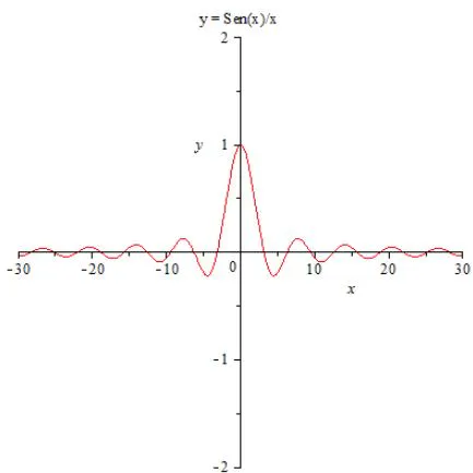
J 0 ( x ) = π 2 x J 1 2 ( x ) = π 2 x 2 π x sin x = sin x x

III. PLOTTING WITH MAPLE

a) Plotting sin ( x ) / x

Figure 2: Plot of sin ( x ) / x

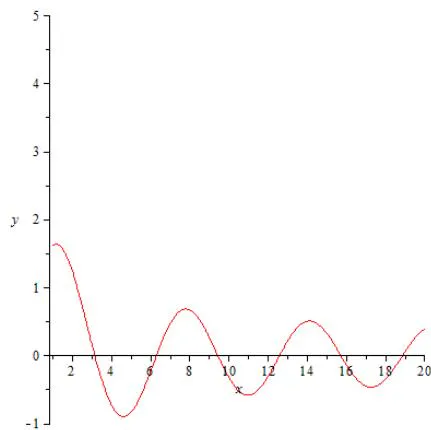
b) Plotting of J ( 1 / 2 )

p l o t ( 2 π x cos ( x 1 4 ( 1 ) π ) + 2 π x cos ( x 1 4 ( 2 ) π ) +
2 π x cos ( x 1 4 ( 3 ) π ) , x = 1.20 , y = 1.5 , d i s c o u n t = t r u e , c o l o r = r e d

Figure 2: Plot of Sin ( 2 / π x ) 2 Sin ( x )

c) Plotting J ( 1 / 2 ) with variations

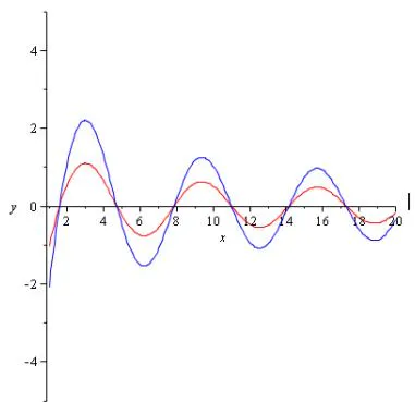
p l o t ( [ 2 π x sin ( x 1 4 ( 1 ) π ) + 2 π x sin ( x 1 4 ( 2 ) π ) + 2 π x sin ( x 1 4 ( 3 ) π ) , 2 ( 2 π x sin ( x 1 4 ( 1 ) π ) + 2 π x sin ( x 1 4 ( 2 ) π ) + 2 π x sin ( x 1 4 ( 3 ) π ) ] , x = 1. . 2 0 , y = 5. . 5 , d i s c o n t = t r u e , c o l o r = [ r e d , b l u e ] )

Figure 4: Plot of Two variations of J ( 1 / 2 )
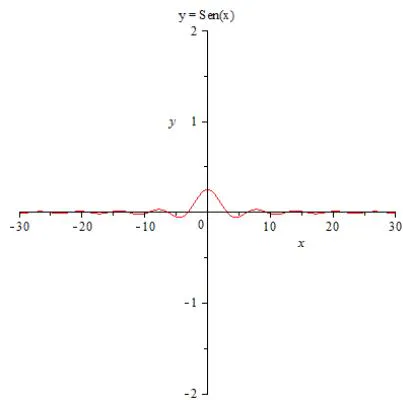
p l o t ( 2 sin ( x ) 8 x ) , x = 30. .30 , y = 2. .2 , d i s c o n t = t r u e ,
t i t l e = y = S e n ( x ) ;
Figure 5: In this plot you can assume a change in the frequency
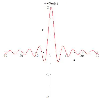
plot ( 2 ( sin ( x ) x ) , x = 3 0. . 3 0 , y = 2. . 2 , discont = true , title = " y = Sen ( x ) ) ;
Figure 6: In this plot you can assume a change in Amplitude

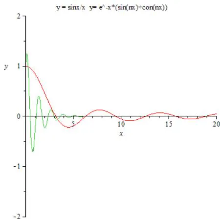
IV. COMPARING BESSEL WITH A LINEAR MODEL UNDERDAMPED

Given that

Figure 7: Bessel J(1/2) vs Over damped

V. ANIMATION OF BESSEL ON MAPLE SOFTWARE

animate(wave, [ u C ( 0 , 3 ) ] , t = 0. . P ( 0 , 3 ) ) ;

1*1234567890

1
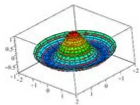
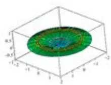
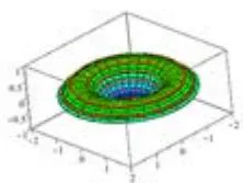
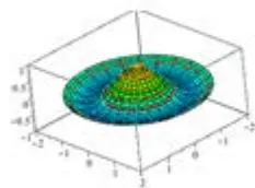
Figure 8: Four snapshots of the Bessel animation

VI. CONCLUSION

A study of Bessel equations can lead us to new applications in acoustics. By changing their parameters, we can determine the ratio between a membrane dimension and the acoustic power it can radiate or the way the membrane will vibrate. For example, we can find analogies between the elasticity of a trampoline jumper and a loudspeaker membrane. We can also study suspension, material thickness, and surfaces and compare them to computer animations which allow us to explore these analogies. Thus, educational institutions with low budgets can make physics experiments on vibration and mechanics at more affordable prices using computer animations. Knowing Bessel equation and its relationship with Helmholtz's formula we can extend the application to the resonance phenomena too.

ACKNOWLEDGMENT

The authors thank Dr. James S. Sochacki for his invaluable assistance and his thorough review of this paper. Dr. Sochacki is a James Madison University Emeritus

Professor in the department of Mathematics and Statistics. Dr. Sochacki is also coauthor of the Parker-Sochacki's algorithm widely for solving systems of ordinary Differential Equations (https://en.wikipedia.org/wiki/Parker%E2%80%93Sochacki_method).

References

6 Cites in Article
  1. Dennis Zill (1982). A First course in Differential Equations with Applications.
  2. Dennis Zill (2022). Advance Engineering Mathematics.
  3. Sunidhi Hanchinmani,Shreya Bellutagi,Basavaraj Madagouda,Nandini Kotagi,Kushali Patil (2018). AUTOMATED HELMET DETECTION AND NUMBER PLATE RECOGNITION USING AI.
  4. A Teboho,Moloi (2022). Spherical Bessel Functions.
  5. Annie Cuyt (2019). High accuracy trigonometric approximations of the real Bessel functions of the First kind.
  6. Elena Shmoylova,Stefan Vorkoetter (2024). Reflections on Maple's History as Told by Stefan Vorkoetter.

Funding

No external funding was declared for this work.

Conflict of Interest

The authors declare no conflict of interest.

Ethical Approval

No ethics committee approval was required for this article type.

Data Availability

Not applicable for this article.

How to Cite This Article

Jose Mujica EE, Ramon A. Mata-Toledo, escuelasuperiordeaudio. 2026. "Obtaining the Sinusoid for Working with Membrane Vibration from the Bessel Differential Equation". Global Journal of Science Frontier Research - F: Mathematics & Decision GJSFR-F Volume 23 (GJSFR Volume 23 Issue F1).

Download Citation

High-impact image of membrane vibration analysis in Bessel differential equation research.
Journal Specifications

Crossref Journal DOI 10.17406/GJSFR

Print ISSN 0975-5896

e-ISSN 2249-4626

Keywords
Classification
GJSFR-F Classification DDC Code: 515.35 LCC Code: QA371
Version of record

v1.2

Issue date
March 3, 2023

Language
English
Experiance in AR

Explore published articles in an immersive Augmented Reality environment. Our platform converts research papers into interactive 3D books, allowing readers to view and interact with content using AR and VR compatible devices.

Read in 3D

Your published article is automatically converted into a realistic 3D book. Flip through pages and read research papers in a more engaging and interactive format.

Article Matrices
Total Views: 490
Total Downloads: 35
All Trends

Request Access

Please fill out the form below to request access to this research paper. Your request will be reviewed by the editorial or author team.
X

This is the heading

Lorem ipsum dolor sit amet, consectetur adipiscing elit. Ut elit tellus, luctus nec ullamcorper mattis, pulvinar dapibus leo.

High-quality academic research articles on global topics and journals.

Obtaining the Sinusoid for Working with Membrane Vibration from the Bessel Differential Equation

Jose EE
Jose EE
Ramon Mata-Toledo
Ramon Mata-Toledo