On Anisotropic Conservative Caginalp Phase-Field System Based on Type III Heat Conduction with Two Temperatures and Periodic Boundary Conditions

Cyr SÃ©raphin Ngamouyih Moussata; Armel Judice Ntsokongo; DieudonnÃ© Ampini

I. INTRODUCTION

The authors studied in [13](see aigain [12]) the following phase-field system, namely,

where, $u$ is the order parameter, $T$ is the relative temperature (defined as $T = \widetilde{T} - T_E$ , where $\widetilde{T}$ is the absolute temperature and $T_E$ is the equilibrium melting temperature), $\alpha$ is the conductive thermal displacement and $f$ is the derivative of a double-well potential $F$ (a typical choice is $F(s) = \frac{1}{4}(s^2 - 1)^2$ , hence the usual cubic nonlinear term $f(s) = s^3 - s$ ). Furthermore, here and below, we set all physical parameters equal to one. This system has been introduced to model phase transition phenomena, such as melting-solidification phenomena, and has been much studied from a mathematical point of view. We refer the reader to, e.g., [4-5, 8-11, 14, 16, 17, 21, 23].

This system is based on the (total Ginzburg-Landau) free energy,

where $\Omega$ is the domain occupied by the system (we assume here that it is a bounded and regular domain of $\mathbb{R}^n$ , $n = 2$ or $n = 3$ , with boundary $\Gamma$ ), and the enthalpy

As far as the evolution equation for the order parameter is concerned, one postulates the relaxation dynamics (with relaxation parameter set equal to one)

where $\frac{D}{Du}$ denotes a variational derivative with respect to $u$ . Then, we have the energy equation

and owing to (1.7),

where $q$ is the heat flux. Assuming finally the usual Fourier law for heat conduction,

we obtain (1.1) and (1.2).

Our aim in this paper is to study the model consisting of the conserved anisotropic to (1.1)-(1.2), namely,

Our aim in this paper is to study the model consisting of the anisotropic conservative equation (1.10) and the temperature equation (1.11). In particular, we obtain the existence and uniqueness of solutions.

II. SETTING OF THE PROBLEM

Find the order parameter $\mathbf{u}:\Omega \times \mathbb{R}^{+}\to \mathbb{R}$ and the terminal displacement $\alpha:\Omega \times \mathbb{R}^{+}\to \mathbb{R}$ such that:

together with periodic boundary conditions

and the initial conditions

We assume that

and we introduce the elliptic operator $A$ defined by

where $H^{-1}(\Omega)$ is the topological dual of $H_{per}^{1}(\Omega)$ . Furthermore, $((.,)$ ) denotes the usual $L^2$ -scalar product, with associated norm $\|. \|$ ; more generally, we denote by $\|. \|_X$ the norm on the Banach space $X$ and we set $\|. \|_{-1} = \| (-\Delta)^{-\frac{1}{2}}. \|$ , $(-\Delta)^{-1}$ denoting the inverse minus Laplace operator with periodic boundary conditions and acting on functions with null average, is a norm in $H^{-1}(\Omega) = H_{per}^{1}(\Omega)'$ which is equivalent to the usual $H^{-1}$ -norm. We can note that

is bilinear, symmetric, continuous and coercive, so that

is indeed well defined. It then follows from elliptic regularity results for linear elliptic operators of order 2 (see [1-2]) that $A$ is a strictly positive, selfadjoint and unbounded linear operator with compact inverse, with domain

where, for $v\in D(A)$

We further note that $D(A^{\frac{1}{2}}) = H_{per}^{1}(\Omega)$ and, for $v \in D(A^{\frac{1}{2}})$ ,

We finally note that (see, e.g., [18]) $v \mapsto (\| Av\|^2 + \langle v \rangle^2)^{\frac{1}{2}}$ defines a norm on $H_{per}^{2}(\Omega)$ which is equivalent to the usual $H^{2}$ -norm on $D(A)$ (resp., $v \mapsto (\| A^{\frac{1}{2}}v\|^2 + \langle v \rangle^2)^{\frac{1}{2}}$ defines a norm on $H_{per}^{1}(\Omega)$ which is equivalent to the usual $H^{1}$ -norm on $D(A^{\frac{1}{2}})$ ), where

being understood that, for $v\in H^{-1}(\Omega)$

and we note that

is a norm on $H^{-1}(\Omega)$ which is equivalent to the usual one. Here, $\Omega = \prod_{i=1}^{n}(0, L_i)$ , $L_i > 0$ , $n = 2$ or $n = 3$ . Furthermore, for a space $W$ we shall denote by $\dot{W}$ the space

Remark 2.1. Actually, the conserved phase-field system usually is endowed with Neumann boundary conditions. In our case, these conditions read

where $\nu$ denotes the unit outer normal.

Remark 2.2. Note that similar properties hold for the operator $-\Delta$ , with obvious changes.

Having this, we rewrite (2.1) as

Furthermore, we assume that the function $f$ satisfies the following conditions:

where, we denote by $F$ the primitive of $f$ vanishing at $s = 0$ ,

Remark 2.3. In particular, these assumptions are satisfied by function

(and, the usual cubic nonlinear term $f(s) = s^3 - s$ ).

Throughout the paper, the same letters $c$ , $c'$ and $c''$ denote (generally positive) constants which may vary from line to line. Similarly, the same letter $Q$ denotes (positive) monotone increasing (with respect to each argument) and continuous functions which may vary from line to line.

III. A PRIORI ESTIMATES

The estimates below are formal, but they can also be justified within a Galerkin scheme for the approximated problem.

We first note that, integrating (formally) (2.8) over $\Omega$ , we have

hence

Furthermore, integrating (2.2) over $\Omega$ , we obtain, in view of (2.7),

It thus follows from (2.4) and (3.2) that

meaning, in particular, that $\left\langle u + \frac{\partial\alpha}{\partial t}\right\rangle$ is a conserved quantity and from (3.1) that

so that

We now assume that

for fixed positive constants $M_1$ et $M_2$ . Thus,

Furthermore, it follows from (3.5) that

We rewrite, in view of (3.4), (2.8) as

and, in view of (3.3) an (3.9) that

Furthermore, we deduce from (2.2) and (3.2) that

We first multiply (3.9) by $\frac{\partial u}{\partial t}$ and obtain, noting that $\left\langle \frac{\partial u}{\partial t} \right\rangle = 0$

We then multiply (2.2) by $\frac{\partial\alpha}{\partial t} -\Delta \frac{\partial\alpha}{\partial t}$ to obtain

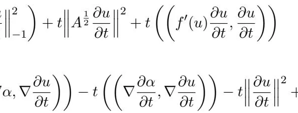
(note indeed that $\left\| \frac{\partial \alpha}{\partial t} - \Delta \frac{\partial \alpha}{\partial t} \right\|^2 = \left\| \frac{\partial \alpha}{\partial t} \right\|^2 + 2 \left\| \nabla \frac{\partial \alpha}{\partial t} \right\|^2 + \left\| \Delta \frac{\partial \alpha}{\partial t} \right\|^2$ ).

Summing finally (3.12) and (3.13), we find a differential equality

satisfies, owing to (2.12),

(here and below, when not specified, the sign of the constants ( $c'$ and $c''$ ) can be arbitrary). Multiplying (3.9) by $\overline{u}$ and have, integrating over $\Omega$ and by parts,

It follows from (2.11) that

from (2.12) and (3.7) that

and from (3.7) that

Therefore, owing again to (3.7) and remembering that $v \mapsto (\| A^{\frac{1}{2}}v\|^{2} + \langle v\rangle^{2})^{\frac{1}{2}}$ is a norm in $H_{per}^{1}(\Omega)$ which is equivalent to the usual $H^{1}$ -norm,

Summing (3.14) and $\delta_1(3.17)$ , where $\delta_1 > 0$ is small enough, we have a differential inequality of the form

satisfies

We multiply (2.8) by $u$ to obtain, owing to (2.9) and (2.10),

Summing (3.18) and $\delta_{2}(3.20)$ , where $\delta_{2} > 0$ is small enough, we obtain a differential inequality of the form

where

satisfies

Now, multiplying (3.10) by $\frac{\partial u}{\partial t}$ , we have

We then multiply (3.11) by $\frac{\partial\overline{\alpha}}{\partial t} -\Delta \frac{\partial\overline{\alpha}}{\partial t}$

(note indeed that $\left\| \frac{\partial \overline{\alpha}}{\partial t} - \Delta \frac{\partial \overline{\alpha}}{\partial t} \right\|^2 = \left\| \frac{\partial \overline{\alpha}}{\partial t} \right\|^2 + 2 \left\| \nabla \frac{\partial \overline{\alpha}}{\partial t} \right\|^2 + \left\| \Delta \frac{\partial \overline{\alpha}}{\partial t} \right\|^2$ ).

Summing finally (3.21), (3.23) and (3.24), we obtain a differential inequality of the form

where

satisfies

We finally assume that $p = 1$ when $n = 3$ and multiply (2.8) by $Au$ to find

We assume that $n = 3$ and $p = 1$ (the case $n = 2$ can be treated in a similar way) and have, owing to (2.12) and Hölder's inequality,

Notes

Therefore,

IV. WELL-POSEDNESS

We have the following result.

Theorem 4.1. We assume that (2.9)-(2.12) hold. Then, for every $(u_0,\alpha_0,\alpha_1)\in (H_{per}^1 (\Omega)\cap L^{2p + 2}(\Omega))\times H_{per}^2 (\Omega)\times H_{per}^2 (\Omega))$ , (2.1)-(2.4) possesses at least one solution $(u,\alpha,\frac{\partial\alpha}{\partial t})$ such that

and

$\forall T > 0$

Furthermore, if $p = 1$ when $n = 3$ , then

Proof. The proof is based on (3.8), (3.25), (3.27) and, e.g., a standard Galerkin scheme.

We have, concerning the uniqueness, the following.

Theorem 4.2. We assume that the assumptions of Theorem 4.1 hold and that $p = 1$ when $n = 3$ and $p \in [1,2]$ when $n = 2$ . Then, the solution obtained in Theorem 4.1 is unique.

Proof. Let $\left(u^{(1)},\alpha^{(1)},\frac{\partial\alpha^{(1)}}{\partial t}\right)$ and $\left(u^{(2)},\alpha^{(2)},\frac{\partial\alpha^{(2)}}{\partial t}\right)$ be two solutions to (2.1)-(2.3) with initial data $(u_0^{(1)},\alpha_0^{(1)},\alpha_1^{(1)})$ and $(u_0^{(2)},\alpha_0^{(2)},\alpha_1^{(2)})$ , respectively, such that

for fixed positive constants $M_{1}$ and $M_2$ .We set

and

We have

We multiply (4.2) by $\frac{\partial u}{\partial t}$ (note that $\left\langle \frac{\partial u}{\partial t} \right\rangle = 0$ ) and obtain

We first assume that $n = 3$ and $p = 1$ . We have

Furthermore, owing to Agmon's inequality,

and, owing to Hölder's inequality,

We now assume that $n = 2$ and we take the most complicated case $p = 2$ . Then, owing to Agmon's inequality and a proper interpolation inequality,

Furthermore, owing to Hölder's inequality,

Finally, we obtain, in both cases, an inequality of the form

Multiplying then (4.3) by $\frac{\partial\alpha}{\partial t} -\Delta \frac{\partial\alpha}{\partial t}$ , we find

Summing finally (4.7) and (4.8), we have, an inequality of the form

$q\geqslant 1$ , where

Then, We deduce from (4.9), (3.8), the estimates obtained in the previous subsection and Gronwall's lemma the uniqueness, as well as the continuous dependence with respect to the initial data.

V. REGULARITY OF SOLUTIONS

We have the following result which gives the existence and uniqueness of more regular solutions.

Theorem 5.1. We assume that the assumptions of Theorem 4.1 hold and that (2.12) is replaced by

Then, if $(u_0,\alpha_0,\alpha_1)\in H_{per}^2 (\Omega)\times H_{per}^3 (\Omega)\times H_{per}^3 (\Omega)$ , the problem possesses a unique solution such that

and

Proof. The proof of uniqueness is obtained by proceeding as in that of Theorem 4.2, noting that, with the higher regularity considered here, no growth assumption on $f$ is needed, owing to the continuous embedding $H_{per}^{2}(\Omega) \subset L^{\infty}(\Omega)$ .

We now turn to the proof of existence and, more precisely, of the further regularity of the solutions.

We multiply (2.8) by $\frac{\partial u}{\partial t}$ , we have

Multiplying then (2.2) by $-\Delta \left(\frac{\partial \alpha}{\partial t} - \Delta \frac{\partial \alpha}{\partial t}\right)$ , we obtain

Summing finally (5.2) and (5.3), we find

It follows from (5.4) and the continuous embedding $H_{per}^{2}(\Omega)\subset \mathcal{C}(\overline{\Omega})$ that

We set

and we deduce from (5.5) that we have an inequality of the form

Let $z$ be the solution to the ordinary differential equation

It follows from the comparison principle that there exists $T_0 = T_0(\| u_0\|_{H_{per}^2 (\Omega)},\| \alpha_0\|_{H_{per}^3 (\Omega)},\| \alpha_1\|_{H_{per}^3 (\Omega)})$ (say, belongin to $(0,\frac{1}{2})$ ) such that

from which it follows, owing also to (3.8) and (3.25), that

We now differentiate (3.9) with respect to times and have, owing to (2.2),

We multiply (5.11) by $t\frac{\partial u}{\partial t}$ and have

which yields, owing to (2.10) and a proper interpolation inequality (see the proof of Theorem 4.2),

It follows from (3.25), (5.12) and Gronwall's lemma that

Next, we multiply (5.11) by $\frac{\partial u}{\partial t}$ and obtain, proceeding similarly,

We deduce from (3.25), (5.14) and Gronwall's lemma that

hence, owing to (5.13),

We rewrite, for $t\geqslant T_0$ fixed, (3.9) as an elliptic equation,

where

satisfies, owing to (3.25) and (5.15),

Multiplying (5.16) by $\overline{u}$ , we find, owing to (2.11) and (5.1),

Multiplying then (5.16) by $Au$ , we have, owing to (2.10),

Combining (5.19) and (5.20), we finally obtain, owing to (3.25) and (5.18),

hence, owing to (5.10),

We now come back to (5.3), from which it follows that

Noting that it follows from (3.25), (5.14) and (5.15) that

we deduce from (3.14), (5.23) and (5.24) that

hence, owing to (3.8), (3.25), (5.10) and (5.22),

which finishes the proof of the theorem.

ACKNOWLEDGEMENTS

The author is thankful to Alain Miranville for helpful discussions. He also wishes to thank an anonymous referee for her/his careful reading of the paper and useful comments.

[1] S. Agmon, Lectures on elliptic boundary value problems, Mathematical Studies. Van Nostrand, New York, 1965.
[2] S. Agmon, A. Douglis and L. Nirenberg, Estimates near the boundary for solutions of elliptic partial differential equations, I, Commun. Pure Appl. Math., 1959, 12, 623-727.
[3] G. Caginalp, Conserved-phase field system: implications for kinetic undercooling, phys. Rev. B, 1988, 38, 789-791.
[4] G. Caginalp, An analysis of a phase-field model of a free boundary, Arch. Rational Mech. Anal., 1986, 92, 205-245.
[5] G. Caginalp and E. Esenturk, Anisotropic phase-field equations of arbitrary order, Discrete Contin. Dyn. Systems S, 2011, 4, 311-350.
[6] X. Chen, G. Caginalp and E. Esenturk Interface conditions for a phase field model with anisotropic and non-local interactions, Arch. Rational Mech. Anal., 2011, 202, 349-372.
[7] G. Giacomin and J.L. Lebowitz, Phase segregation dynamics in particle systems with long range interaction I. Macroscopic limits, J. Statist. Phys., 1997, 87, 37-61.
[8] L. Cherfils, A. Miranville, S. Peng and W. Zhang Higher-order generalized Cahn-Hilliard equation, Electron. J. Qualitative Theory Diff. Eqns., 2017, 9, 1-22.
[9] L. Cherfils, A. Miranville and S.Peng, Higher-order models in phase separation, J. Appl. Anal. Comput., 2017, 7, 39-56.
[10] L. Cherfils, A. Miranville and S. Peng, Higher-order Allen-Cahn models with logarithmic nonlinear terms, Advances in dynamical systems and control, 69, 247-263, 2016.
[11] A. Miranville, Higher-order Anisotropic Caginalp Phase-Field systems, Mediterr. J. Math., 2016, 13, 4519–4535.
[12] A. Miranville and A.J. Ntsokongo, On the anisotropic Caginalp phase-field type models with singular nonlinear terms, Journal of Applied Analysis and Computation, 655-274, 8, 2018.
[13] A. Miranville and R. Quintanilla, A Caginalp phase-field system based on type III heat conduction with two temperatures, Quart. Appl. Math., 2016, 74, 375-398.
[14] A. Miranville and A. Pietrus, A new formulation of the Cahn-Hilliard equation, Nonlinear Analysis: Real World Applications, 2006, 7, 285-307.
[15] A.J. Ntsokongo, On higher-order anisotropic Caginalp phase-field systems with polynomial nonlinear terms, J. Appl. Anal. Comput., 2017, 7, 992-1012.
[16] A. Makki and A. Miranville, Existence of solutions for anisotropic Cahn-Hilliard and Allen-Cahn systems in higher space dimensions, Discrete and Continuous Dynamical Systems Series S, 2016, 9, 759-775.
[17] R. Temam, Infinite-dimensional dynamical systems in mechanics and physics, Second edition, Applied Mathematical Sciences, vol. 68, Springer-Verlag, New York, 1997.
[18] J.E. Taylor, Mean curvature and weighted mean curvature, Acta Metall. Mater., 1992, 40, 1475-1495.
[19] J.W. Cahn and J. E Hilliard, Free energy of a nonuniform I. Interfacial free energy, J. Chem. Phys., 1958, 2, 258-267.
[20] R. Kobayishi, Modelling and numerical simulations of dentritic chrystal growth, Phys. D, 1993, 63, 410-423.
[21] A. Kostianko and S. Zelik, Inertial manifolds for the 3D Cahn-Hilliard equation with periodic boundary conditions, Commun. Pure Appl. Anal, 2015, 14, 2069-2094.
[22] C.I. Christov and P.M. Jordan, Heat conduction paradox involving second-sound propagation in moving media, Phys. Review Letters, 2005, 94, 154-301.
[23] H. Gajewski and K. Zacharias, Global behaviour of a reaction-diffusion system modelling chemotaxis., Math. Nachr., 1998, 195, 77-114.
[24] P.J. Chen, M.E. Gurtin and W.O. Williams, A note on non-simple heat conduction, J. Appl. Math. Psys. (ZAMP) 1968, 19, 969-970.
[25] R. Quintanilla, A well-posed problem for the three-dual-phase-lag heat conduction, J. Thermal Stresses, 2009, 32, 1270-1278.

References

23 Cites in Article
1.S Agmon (1965). Unknown Title.
2.S Agmon,A Douglis,L Nirenberg (1959). Estimates near the boundary for solutions of elliptic partial differential equations satisfying general boundary conditions. I. Communications on Pure and Applied Mathematics, 12(4), 623-727.
3.G Caginalp (1988). Conserved-phase field system: Implications for kinetic undercooling. Physical Review B, 38(1), 789-791.
4.Gunduz Caginalp (1986). An analysis of a phase field model of a free boundary. Archive for Rational Mechanics and Analysis, 92(3), 205-245.
5.Giambattista Giacomin,Joel Lebowitz (1997). Phase segregation dynamics in particle systems with long range interactions. I. Macroscopic limits. Journal of Statistical Physics, 87(1-2), 37-61.
6.Laurence Cherfils,Alain Miranville,Shuiran Peng,Wen Zhang (2017). Higher-order generalized Cahn–Hilliard equations. Electronic Journal of Qualitative Theory of Differential Equations, 9(9), 1-22.
7.Laurence Cherfils,Alain Miranville,Shuiran Peng (2017). Higher-order anisotropic models in phase separation. Advances in Nonlinear Analysis, 8(1), 278-302.
8.Laurence Cherfils,Alain Miranville,Shuiran Peng (2016). Higher-Order Allen–Cahn Models with Logarithmic Nonlinear Terms. Studies in Systems, Decision and Control, 69, 247-263.
10.A Miranville,A Ntsokongo (2018). On the anisotropic Caginalp phase-field type models with singular nonlinear terms. Journal of Applied Analysis and Computation, 655-274.
11.Alain Miranville,Ramon Quintanilla (2016). A Caginalp phase-field system based on type III heat conduction with two temperatures. Quarterly of Applied Mathematics, 74(2), 375-398.
12.Alain Miranville,Alain Piétrus (2006). A new formulation of the Cahn–Hilliard equation. Nonlinear Analysis: Real World Applications, 7(2), 285-307.
13.A Ntsokongo (2017). On higher-order anisotropic Caginalp phase-field systems with polynomial nonlinear terms. J. Appl. Anal. Comput, 7, 992-1012.
14.A Makki,A Miranville (2016). Existence of solutions for anisotropic Cahn-Hilliard and Allen-Cahn systems in higher space dimensions. Discrete and Continuous Dynamical Systems Series S, 9, 759-775.
15.Roger Temam (1997). Infinite-Dimensional Dynamical Systems in Mechanics and Physics.
16.J Taylor (1992). II—mean curvature and weighted mean curvature. Acta Metallurgica et Materialia, 40(7), 1475-1485.
17.John Cahn,John Hilliard (1958). Free Energy of a Nonuniform System. I. Interfacial Free Energy. The Journal of Chemical Physics, 28(2), 258-267.
18.R Kobayishi (1993). Modelling and numerical simulations of dentritic chrystal growth. Phys. D, 63, 410-423.
19.A Kostianko,S Zelik (2015). Inertial manifolds for the 3D Cahn-Hilliard equation with periodic boundary conditions. Commun. Pure Appl. Anal, 14, 2069-2094.
20.C Christov,P Jordan (2005). Heat Conduction Paradox Involving Second-Sound Propagation in Moving Media. Physical Review Letters, 94(15), 154-301.
21.Herbert Gajewski,Klaus Zacharias,Konrad Gröger (1998). Global Behaviour of a Reaction‐Diffusion System Modelling Chemotaxis. Mathematische Nachrichten, 195(1), 77-114.
22.Peter Chen,William Williams (1968). A note on non-simple heat conduction. Zeitschrift für angewandte Mathematik und Physik ZAMP, 19(6), 969-970.
23.Ramon Quintanilla (2009). A Well-Posed Problem for the Three-Dual-Phase-Lag Heat Conduction. Journal of Thermal Stresses, 32(12), 1270-1278.
Explore published articles in an immersive Augmented Reality environment. Our platform converts research papers into interactive 3D books, allowing readers to view and interact with content using AR and VR compatible devices.
Your published article is automatically converted into a realistic 3D book. Flip through pages and read research papers in a more engaging and interactive format.