## I. INTRODUCTION The partial differential equations of fractional order (FPDEs) have been widely employed in recent years to explain a wide range of physical effects and complicated nonlinear phenomena. This is because they accurately describe nonlinear phenomena in the fields of fluid mechanics, viscoelasticity, electrical chemistry, quantum biology, physics, and engineering mechanics [1]-[6] as well as other scientific domains. As a result, the research of PDEs has received a lot of interest as many physical events may be explained using the idea of fractional derivatives and integrals [7]-[9]. Add to that, when the exact solutions to the majority of FPDEs are difficult to find, analytical and numerical methods [10]-[29] which are proposed and developed by many authors must be used. Lie symmetry analysis is extremely important in many fields of science, particularly in integrable systems with an infinite number of symmetries. Thus, Lie symmetry analysis is regarded as one of the most effective methods for obtaining analytical solutions to nonlinear partial differential equations (NLPDEs). Also, many FPDEs have been studied using this analysis [30]-[36]. Add to that, this analysis is used to build conservation laws, which are crucial in the study of nonlinear physical phenomena. Conservation laws are mathematical formulations state that the total amount of a certain physical quantity remains constant as a physical system evolves. Furthermore, conservation laws are used in the development of numerical methods to establish the existence and uniqueness of a solution. There are many studies that discuss conservation laws for time FPDEs, which are mentioned in the references [37]-[43]. In this article, we focus on the following time-fractional MZKB equation of the form: $$ \partial_ {t} ^ {\alpha} q + \kappa_ {1} \sqrt {q} q _ {x} + \kappa_ {2} q _ {x x x} + \kappa_ {3} \left(q _ {x y y} + q _ {x z z}\right) + \kappa_ {4} q _ {x x} = 0, \tag {1} $$ where $\partial_t^\alpha$ is the fractional derivative of order $\alpha$ (with $0 < \alpha < 1$ ), $\kappa_i(i = 0,1,\dots,4)$ are respectively the dispersion, non linearity, mixed derivative, and dissipation. The $q(x,y,z,t)$ is the potential function of space $x$, $y$, $z$ and time $t$. If $\alpha = 1$, Eq. (1) is reduced to the classical MZKB equation [44, 45], which describes the nonlinear plasma dust ion acoustic waves DIAWs in a magnetized dusty plasma and it is derived using the standard reductive perturbation technique in small amplitude. The article is organized as follows: The introduction is presented in Section 1. In Section 2, some definitions and description of Lie symmetry analysis for fractional partial differential equations (FPDEs) are briefly presented. Lie symmetry analysis and similarity reduction of the Eq. (1) are obtained in Section 3. We construct two sets of analytical solutions for Eq. (1) by using fractional sub-equation method and extended Kudryashov method in Section 4 and 5 respectively. In Section 6, the conservation laws of the Eq. (1) are obtained. Finally, the discussions and conclusions of this article are presented in Section 7. ## II. PRELIMINARIES Here in this section, we focus on some of the concepts that revolve around the subject of our article Definition 1: Let $\alpha >0$. The operator $I^{\alpha}$ defined by $$ I ^ {\alpha} f (t) = \frac {1}{\Gamma (\alpha)} \int_ {0} ^ {t} (t - s) ^ {\alpha - 1} f (s) d s, \tag {2} $$ is called the Riemann-Liouville (R-L) fractional integral operator of order $\alpha$, and $\Gamma(.)$ denotes the gamma function. Definition 2: Let $\alpha >0$. The operator $D_t^\alpha$ is defined by $$ D _ {t} ^ {\alpha} f (t) = \left\{ \begin{array}{l l} \frac{1}{\Gamma (n - \alpha)} \frac{d ^ {n}}{d t ^ {n}} \int_ {0} ^ {t} (t - s) ^ {n - \alpha - 1} f (s) d s & \text{if } n - 1 < \alpha < n, n \in N, \\ \frac{d ^ {n} f (t)}{d t ^ {n}} & \text{if } \alpha = n, n \in N, \end{array} \right. \tag{3} $$ is called the R-L fractional partial derivative [7, 8]. ### a) Description of Lie symmetry analysis Let's consider the symmetry analysis for a FPDE of the form $$ D _ {t} ^ {\alpha} q (x, y, z, t) = G (x, y, z, t, q, q _ {x}, q _ {t}, q _ {y}, q _ {z}, q _ {x x}, q _ {x y}, \dots), \quad 0 < \alpha < 1. \tag {4} $$ Now, let Eq. (4) is invariant under the following one-parameter Lie group of point transformation acting on both the dependent and independent variables, given as $$ \bar {x} = x + \varepsilon \xi (x, y, z, t) + O (\varepsilon^ {2}), $$ $$ \bar {y} = y + \varepsilon \zeta (x, y, z, t) + O (\varepsilon^ {2}), $$ $$ \bar {z} = z + \varepsilon \nu (x, y, z, t) + O (\varepsilon^ {2}), $$ $$ \bar {t} = t + \varepsilon \tau (x, y, z, t) + O (\varepsilon^ {2}), $$ $$ \bar {q} = q + \varepsilon \eta (x, y, z, t) + O (\varepsilon^ {2}), $$ $$ D _ {t} ^ {\alpha} \bar {q} = D _ {t} ^ {\alpha} q + \varepsilon \eta_ {\alpha} ^ {0} (x, y, z, t) + O (\varepsilon^ {2}), $$ $$ \frac {\partial \bar {q}}{\partial \bar {x}} = \frac {\partial q}{\partial x} + \varepsilon \eta^ {x} (x, y, z, t) + O \left(\varepsilon^ {2}\right), \tag {5} $$ $$ \frac{\partial^ {2} \bar{q}}{\partial \bar{x} ^ {2}} = \frac{\partial^ {2} q}{\partial x ^ {2}} + \varepsilon \eta^ {x x} (x, y, z, t) + O (\varepsilon^ {2}), $$ $$ \begin{array}{l} \frac{\partial^ {3} \bar{q}}{\partial \bar{x} ^ {3}} = \frac{\partial^ {3} q}{\partial x ^ {3}} + \varepsilon \eta^ {x x x} (x, y, z, t) + O (\varepsilon^ {2}), \\\frac{\partial^ {3} \bar{q}}{\partial \bar{x} \partial \bar{y} ^ {2}} = \frac{\partial^ {3} q}{\partial x \partial y ^ {2}} + \varepsilon \eta^ {x y y} (x, y, z, t) + O (\varepsilon^ {2}), \\\frac{\partial^ {3} \bar{q}}{\partial \bar{x} \partial \bar{z} ^ {2}} = \frac{\partial^ {3} q}{\partial x \partial z ^ {2}} + \varepsilon \eta^ {x z z} (x, y, z, t) + O (\varepsilon^ {2}), \\\end{array} $$ Notes where $\varepsilon \ll 1$ is the Lie group parameter and $\xi, \zeta, \nu, \tau, \eta$ are the infinitesimals of the transformations for dependent and independent variables respectively. The explicit expressions of $\eta^x$, $\eta^{xx}$, $\eta^{xxx}$, $\eta^{xyy}$, $\eta^{xzz}$ are given by $$ \eta^{x} = D_{x}(\eta) - q_{x}D_{x}(\xi) - q_{y}D_{x}(\zeta) - q_{z}D_{x}(\nu) - q_{t}D_{x}(\tau), $$ $$ \eta^{xx} = D_{x}\left(\eta^{x}\right) - q_{xx}D_{x}\left(\xi\right) - q_{xy}D_{x}\left(\zeta\right) - q_{xz}D_{x}\left(\nu\right) - q_{xt}D_{x}\left(\tau\right), $$ $$ \eta^{xxx} = D_{x}\left(\eta^{xx}\right) - q_{xxx}D_{x}\left(\xi\right) - q_{xx y}D_{x}\left(\zeta\right) - q_{xxz}D_{x}\left(\nu\right) - q_{xxt}D_{x}\left(\tau\right), $$ $$ \eta^{xyy} = D_{x}\left(\eta^{yy}\right) - q_{xyy}D_{x}\left(\xi\right) - q_{xyz}D_{x}\left(\zeta\right) - q_{xyt}D_{x}\left(\nu\right) - q_{xyt}D_{ x}\left(\tau\right), $$ $$ \eta^{xzz} = D_{x}\left(\eta^{zz}\right) - q_{xxz}D_{x}\left(\xi\right) - q_{xyz}D_{x}\left(\zeta\right) - q_{xzz}D_{x}\left(\nu\right) - q_{xzt}D_{x}\left(\tau\right), $$ where $D_x$, $D_y$, $D_z$, and $D_t$ are the total derivatives with respect to $x$, $y$, $z$, and $t$ respectively that are defined for $x^1 = x$, $x^2 = y$, $x^3 = z$ as $$ D _ {x j} = \frac {\partial}{\partial x ^ {j}} + q _ {j} \frac {\partial}{\partial q} + q _ {j k} \frac {\partial}{\partial q _ {k}} + \dots , \quad j, k = 1, 2, 3, \dots $$ where $q_{j} = \frac{\partial q}{\partial x^{j}}$ $q_{jk} = \frac{\partial^2q}{\partial x^k}$ and so on. The corresponding Lie algebra of symmetries consists of a set of vector fields of the form $$ V = \xi \frac {\partial}{\partial x} + \zeta \frac {\partial}{\partial y} + \nu \frac {\partial}{\partial z} + \tau \frac {\partial}{\partial t} + \eta \frac {\partial}{\partial u}. $$ The invariance condition of Eq. (4) under the infinitesimal transformations is given as $$ P r ^ {(n)} \left. V (\Delta) \mid_ {\Delta = 0} = 0, \quad n = 1, 2, 3, \dots \right. $$ where $$ \Delta := D _ {t} ^ {\alpha} q (x, y, z, t) - G (x, y, z, t, q, q _ {x}, q _ {t}, q _ {y}, q _ {z}, q _ {x x}, q _ {x y}, \dots). $$ Also, the invariance condition gives $$ \tau (x, y, z, t, u) \mid_ {t = 0} = 0. \tag {7} $$ The $\alpha$ th extended infinitesimal related to RL fractional time derivative with Eq. (7) can be represented as follows $$ \eta_\alpha^0 = D_t^\alpha(\eta) + \xi D_t^\alpha(q_x) - D_t^\alpha(\xi q_x) + \zeta D_t^\alpha(q_y) - D_t^\alpha(\zeta q_y) + \nu D_t^\alpha(q_z) \tag{8} \- D_t^\alpha(\nu q_z) + D_t^\alpha(D_t(\tau)q) - D_t^{\alpha+1}(\tau q) + \tau D_t^{\alpha+1}(q), $$ where $D_t^\alpha$ is the total fractional derivative operator and by using the generalized Leibnitz rule $$ D_{t}^\alpha \Big (f(t) g(t) \Big) = \sum_{n = 0}^\infty \binom{\alpha}{n} D_{t}^{\alpha - n} f(t) D_{t}^{n} g(t), \binom{\alpha}{n} = \frac{(- 1) ^{n - 1} \alpha \Gamma (n - \alpha)}{\Gamma (1 - \alpha) \Gamma (n + 1)} $$ By applying the Leibnitz rule, Eq. (8) becomes $$ \begin{array}{l} \eta_ {\alpha} ^ {0} = D _ {t} ^ {\alpha} (\eta) - \alpha D _ {t} ^ {\alpha} (\tau) \frac {\partial^ {\alpha} q}{\partial t ^ {\alpha}} - \sum_ {n = 1} ^ {\infty} \binom {\alpha} {n} D _ {t} ^ {n} (\xi) D _ {t} ^ {\alpha - n} q _ {x} - \sum_ {n = 1} ^ {\infty} \binom {\alpha} {n} D _ {t} ^ {n} (\zeta) D _ {t} ^ {\alpha - n} q _ {y} \\- \sum_ {n = 1} ^ {\infty} \binom {\alpha} {n} D _ {t} ^ {n} (\nu) D _ {t} ^ {\alpha - n} q _ {z} - \sum_ {n = 1} ^ {\infty} \binom {\alpha} {n + 1} D _ {t} ^ {n + 1} (\xi) D _ {t} ^ {\alpha - n} q. \tag {9} \\\end{array} $$ Now by using the chain rule for the compound function which is defined as follows $$ \frac {d ^ {n} \phi (h (t))}{d t ^ {n}} = \sum_ {k = 0} ^ {n} \sum_ {r = 0} ^ {k} \left( \begin{array}{c} k \\r \end{array} \right) \frac {1}{k !} \big [ - h (t) \big ] ^ {r} \frac {d ^ {n}}{d t ^ {n}} \big [ - h (t) ^ {k - r} \big ] \times \frac {d ^ {k} \phi (h)}{d h ^ {k}}. $$ By applying this rule and the generalized Leibnitz rule with $f(t) = 1$, we have $$ D _ {t} ^ {\alpha} (\eta) = \frac {\partial^ {\alpha} \eta}{\partial t ^ {\alpha}} + \eta_ {q} \frac {\partial^ {\alpha} q}{\partial t ^ {\alpha}} - q \frac {\partial^ {\alpha} \eta_ {q}}{\partial t ^ {\alpha}} + \sum_ {n = 1} ^ {\infty} \left( \begin{array}{c} \alpha \\n \end{array} \right) \frac {\partial^ {n} \eta_ {q}}{\partial t ^ {n}} D _ {t} ^ {\alpha - n} (q) + \mu , $$ where $$ \mu = \sum_{n=2}^\infty \sum_{m=2}^n \sim_{k=2}^{m} \sum_{r=0}^{k-1} \binom{\alpha}{n} \binom{n}{m} \binom{k}{r} \frac{1}{k!} \times \frac{t^{n-\alpha}}{\Gamma(n+1-\alpha)} [-q]^r \frac{\partial^m}{\partial t^m} [q^{k-r}] \frac{\partial^{n-m+k} \eta}{\partial t^{n-m} \partial q^k}. $$ Therefore, Eq. (9) yields $$ \begin{array}{l} \eta_ {\alpha} ^ {0} = \frac{\partial^ {\alpha} \eta}{\partial t ^ {\alpha}} + (\eta_ {q} - \alpha D _ {t} ^ {\alpha} (\tau)) \frac{\partial^ {\alpha} q}{\partial t ^ {\alpha}} - q \frac{\partial^ {\alpha} \eta_ {q}}{\partial t ^ {\alpha}} + \mu + \sum_ {n = 1} ^ {\infty} \left[ \binom{\alpha} {n} \frac{\partial^ {\alpha} \eta_ {q}}{\partial t ^ {\alpha}} - \binom{\alpha} {n + 1} D _ {t} ^ {n + 1} (\tau) \right] D _ {t} ^ {\alpha - n} (q) \tag{10} \\+ \sum_ {n = 1} ^ {\infty} \left(\alpha\right) D _ {t} ^ {n} (\xi) D _ {t} ^ {\alpha - n} q _ {x} - \sum_ {n = 1} ^ {\infty} \binom{\alpha} {n} D _ {t} ^ {n} (\zeta) D _ {t} ^ {\alpha - n} q _ {y} - \sum_ {n = 1} ^ {\infty} \binom{\alpha} {n} D _ {t} ^ {n} (\nu) D _ {t} ^ {\alpha - n} q _ {z}. \\\end{array} $$ Definition 3: The function $q = \theta(x, y, z, t)$ is an invariant solution of Eq. (4) associated with the vector field $W$, such that 1. $q = \theta (x,y,z,t)$ is an invariant surface of Eq. (4), this means $$ V \theta = 0 \Leftrightarrow \left(\xi \frac {\partial}{\partial x} + \zeta \frac {\partial}{\partial y} + \nu \frac {\partial}{\partial z} + \tau \frac {\partial}{\partial t} + \eta \frac {\partial}{\partial u}\right) \theta = 0, $$ #### 2. $q = \theta (x,y,z,t)$ satisfies Eq.4 ## III. LIE SYMMETRY ANALYSIS AND SIMILARITY REDUCTION OF Eq.(1) In this section, we implemented Lie group method for Eq. (1) and then, used these symmetries to reduce Eq. (1) to be a FODE as shown in the next two subsections ### a) Lie symmetry analysis for Eq. (1) Let us consider Eq. (1) is an invariant under Eq. (5), we get $$ \partial_ {t} ^ {\alpha} \bar{q} + \kappa_ {1} \sqrt{\bar{q}} \bar{q} _ {x} + \kappa_ {2} \bar{q} _ {x x x} + \kappa_ {3} (\bar{q} _ {x y y} + \bar{q} _ {x z z}) + \kappa_ {4} \bar{q} _ {x x} = 0, $$ such that $q = q(x,y,z,t)$ satisfies Eq. (1), then using the point transformations Eq. (5) in Eq. (11), we get the invariant equation $$ \eta_ {\alpha} ^ {0} + \kappa_ {1} \sqrt{q} \, \eta^ {x} + \frac{\kappa_ {1}}{2 \sqrt{q}} \, \eta \, q_ {x} + \kappa_ {2} \, \eta^ {xxx} + \kappa_ {3} \, \left(\eta^ {xyy} + \eta^ {xzz}\right) + \kappa_ {4} \, \eta^ {xx} = 0, \tag{12} $$ By substituting Eq. (6) and Eq. (10) into Eq. (12), grouping the coefficients of all derivatives and various powers of $u$ and equating them to zero we get an algebraic system of equations. Solving this system, we obtain a set of infinitesimal symmetries as below: Case 1: When $\kappa_{i} \neq 0$, $i = 1,2,3$, $\kappa_{4} = 0$ $$ \tau = \frac{3}{2\alpha} c_{1} t + c_{2}, \quad \xi = \frac{1}{2} c_{1} x + c_{3}, \quad \zeta = \frac{1}{2} c_{1} y + c_{4}, \quad \nu = \frac{1}{2} c_{1} z + c_{5}, \quad \eta = -2 c_{1} q, \tag{13} $$ where $c_{i}$, $i = 1,2,3,4,5$ are arbitrary constants. Thus, the infinitesimal generator of Eq. (1) can be expressed as follows $$ V = \left(\frac{3}{2\alpha} c_1 t + c_2\right) \frac{\partial}{\partial t} + \left(\frac{1}{2} c_1 x + c_3\right) \frac{\partial}{\partial x} + \left(\frac{1}{2} c_1 y + c_4\right) \frac{\partial}{\partial y} + \left(\frac{1}{2} c_1 z + c_5\right) \frac{\partial}{\partial z} - 2 c_1 q \frac{\partial}{\partial q}. $$ which can be spanned by the five vector fields listed below. $$ V _ {1} = \frac {\partial}{\partial t}, \quad V _ {2} = \frac {\partial}{\partial x}, \quad V _ {3} = \frac {\partial}{\partial y}, \quad V _ {4} = \frac {\partial}{\partial z}, \tag {14} $$ $$ V _ {5} = \frac{3 t}{2 \alpha} \frac{\partial}{\partial t} + \frac{x}{2} \frac{\partial}{\partial x} + \frac{y}{2} \frac{\partial}{\partial y} + \frac{z}{2} \frac{\partial}{\partial z} - 2 q \frac{\partial}{\partial q}. $$ Case 2: When $\kappa_{i} \neq 0$, $i = 1,2,3,4$ $$ \tau = c _ {6}, \qquad \xi = c _ {7}, \qquad \zeta = c _ {8}, \qquad \nu = c _ {9}, \qquad \eta = 0, $$ hence, there are four vector fields as below $$ V _ {6} = \frac {\partial}{\partial t}, \quad V _ {7} = \frac {\partial}{\partial x}, \quad V _ {8} = \frac {\partial}{\partial y}, \quad V _ {9} = \frac {\partial}{\partial z}. \tag {15} $$ # b) The In this part of the article, we used the symmetries defined by Eq. (14) and Eq. (15) to construct the similarity reduction for Eq. (1) as presented in the next cases Case 1: For $V_{1} = \frac{\partial}{\partial t}$, $\dot{V}_{2} = \frac{\partial}{\partial x}$, $V_{3} = \frac{\partial}{\partial y}$, $V_{4} = \frac{\partial}{\partial z}$, $V_{5} = \frac{3t}{2\alpha}\frac{\partial}{\partial t} +\frac{x}{2}\frac{\partial}{\partial x} +\frac{y}{2}\frac{\partial}{\partial y} +\frac{z}{2}\frac{\partial}{\partial z} -2q\frac{\partial}{\partial q}$ with $\kappa_4 = 0$ we have a set of characteristic equations that arranged in the following subcases Case 1.1: $V_{1} = \frac{\partial}{\partial t}$ we have a characteristic equation of the form $$ \frac{dx}{0} = \frac{dy}{0} = \frac{dz}{0} = \frac{dt}{1} = \frac{dq}{0}. $$ by integrating this equation and appoint the solutions $q$ as function of the dependent variables $x, y, z$, that is $$ q (x, y, z, t) = \phi_ {1} (x, y, z), $$ this implies $\frac{\partial^{\alpha}q}{\partial t^{\alpha}} = 0$ and Eq. (1) becomes $$ \kappa_1\sqrt{\phi_1(x,y,z)}\frac{d\phi_1(x,y,z)}{dx} + \kappa_2\frac{d^3\phi_1(x,y,z)}{dx^3} + \kappa_3\left(\frac{d^3\phi_1(x,y,z)}{dxdydy} + \frac{d^3\phi_1(x,y,z)}{dxdzdz}\right) = 0. $$ Case 1.2: For $V_{2} = \frac{\partial}{\partial x}$ we have a characteristic equation of the form $$ {\frac {d x}{1}} = {\frac {d y}{0}} = {\frac {d z}{0}} = {\frac {d t}{0}} = {\frac {d q}{0}}, $$ by solving this equation we have $q(x,y,z,t) = \Phi_2(y,z,t)$ which makes all the derivatives of $u(x,y,z,t)$ with respect to $x$ equal to zero and where $B_0$ is a constant Case 1.3: For $V_{3} = \frac{\partial}{\partial y}$ the characteristic equation is of the form $$ \frac{dx}{0} = \frac{dy}{1} = \frac{dz}{0} = \frac{dt}{0} = \frac{dq}{0}, $$ thus $q(x,y,z,t) = \Phi_3(x,z,t)$ and all the derivatives of $q(x,y,z,t)$ with respect to $y$ equal to zero, therefore $$ \frac{\partial^{\alpha} \Phi_{3}(x,z,t)}{\partial t^{\alpha}} + \kappa_{1} \sqrt{\Phi_{3}(x,z,t)} \frac{d \Phi_{3}(x,z,t)}{d x} + \kappa_{2} \frac{d^{3} \Phi_{3}(x,z,t)}{d x^{3}} + \kappa_{3} \frac{d^{3} \Phi_{3}(x,z,t)}{d x \, d z \, d z} = 0 $$ Case 1.4: For $V_{4} = \frac{\partial}{\partial z}$ the characteristic equation is of the form $$ \frac{dx}{0} = \frac{dy}{0} = \frac{dz}{1} = \frac{dt}{0} = \frac{dq}{0}, $$ thus $q(x,y,z,t) = \Phi_4(x,y,t)$ and all the derivatives of $q(x,y,z,t)$ with respect to $z$ equal to zero, therefore $$ \frac{\partial^{\alpha}\Phi_{4}(x,y,t)}{\partial t^{\alpha}} + \kappa_{1}\sqrt{\Phi_{4}(x,y,t)}\frac{d\Phi_{4}(x,y,t)}{dx} + \kappa_{2}\frac{d^{3}\Phi_{4}(x,y,t)}{dx^{3}} + \kappa_{3}\frac{d^{3}\Phi_{4}(x,y,t)}{dxdydy} = 0 $$ Case 1.5: For $V_{5} = \frac{3t}{2\alpha}\frac{\partial}{\partial t} +\frac{x}{2}\frac{\partial}{\partial x} +\frac{y}{2}\frac{\partial}{\partial y} +\frac{z}{2}\frac{\partial}{\partial z} -2q\frac{\partial}{\partial q}$, the characteristic equation becomes $$ \frac {d x}{x / 2} = \frac {d y}{y / 2} = \frac {d z}{z / 2} = \frac {d t}{3 t / 2 \alpha} = \frac {d q}{- 2 q}. $$ Where solving this equation we can get the next similarity variables and similarity solution for Eq. (1) as below $$ \gamma_ {1} = x t ^ {- \frac {\alpha}{3}}, \quad \gamma_ {2} = y t ^ {- \frac {\alpha}{3}}, \quad \gamma_ {3} = z t ^ {- \frac {\alpha}{3}}, \quad q = t ^ {- \frac {4}{3} \alpha} \phi (\gamma_ {1}, \gamma_ {2}, \gamma_ {3}). \tag {17} $$ By using the above transformation, Eq. (1) can be turned into a nonlinear FODE with a set of independent variable $\gamma^{\prime}s$. Consequently, one can conclude the next theorem. Theorem 1: The transformation Eq. (17) reduces the time-fractional generalized Z-K Eq. (1) to the following equation $$ \left(P_{\frac{3}{\alpha}, \frac{3}{\alpha}, \frac{3}{\alpha}}^{1 - \frac{7\alpha}{3}, \alpha} \phi\right)(\gamma_1, \gamma_2, \gamma_3) + \kappa_1 \sqrt{\phi} \phi_{\gamma_1} + \kappa_2 \phi_{\gamma_1 \gamma_1 \gamma_1} + \kappa_3 \left(\phi_{\gamma_1 \gamma_2 \gamma_2} + \phi_{\gamma_1 \gamma_3 \gamma_3}\right) = 0, $$ with the E-K fractional differential operator $\left(P_{\beta}^{\tau, \alpha} \phi\right)(\gamma_1, \gamma_2, \gamma_3)$ which is defined as $$ \left(P_{\beta_1,\beta_2,\beta_3}^{\tau,\alpha} \phi\right) (\gamma_1,\gamma_2,\gamma_3) = \prod_{j=0}^{n-1} \left(\tau + j - \frac{1}{\beta_1} \gamma_1 \frac{\partial}{\partial \gamma_2} - \frac{1}{\beta_2} \gamma_2 \frac{\partial}{\partial \gamma_2} - \frac{1}{\beta_3} \gamma_3 \frac{\partial}{\partial \gamma_3}\right) \left(K_{\beta_1,\beta_2,\beta_3}^{\tau+\alpha,n-\alpha} \phi\right) (\gamma_1,\gamma_2,\gamma_3), $$ where $n = \left\{ \begin{array}{ll}|\alpha | + 1, & n\notin N,\\ \alpha, & n\in N, \end{array} \right.$ (19) $$ \left(K _ {\beta_ {1}, \beta_ {2}, \beta_ {3}} ^ {\tau + \alpha , n - \alpha} \phi\right) (\gamma_ {1}, \gamma_ {2}, \gamma_ {3}) = \left\{ \begin{array}{l l} \frac{1}{\Gamma (\alpha)} \int_ {1} ^ {\infty} (\Theta - 1) ^ {\alpha - 1} \Theta^ {- (\tau + \alpha)} \phi \left(\gamma_ {1} \Theta^ {\frac{1}{\beta_ {1}}}, \gamma_ {2} \Theta^ {\frac{1}{\beta_ {2}}}, \gamma_ {3} \Theta^ {\frac{1}{\beta_ {3}}}\right) d \Theta , & \quad \alpha > 0, \\ \phi (\gamma_ {1}, \gamma_ {2}, \gamma_ {3}), & \quad \alpha = 0, \end{array} \right. $$ is the E-K fractional integral operator. The proof of theorem 1: Depending on the definition of the R-L fractional derivatives provided with $n - 1 < \alpha < 1$, $n = 1,2,3,\ldots$, then we have $$ \partial_ {t} ^ {\alpha} q = \frac {\partial^ {n}}{\partial t ^ {n}} \left[ \frac {1}{\Gamma (n - \alpha)} \int_ {1} ^ {t} (t - g) ^ {n - \alpha - 1} g ^ {- \frac {1}{3} \alpha} \phi \left(\gamma_ {1} g ^ {- \frac {\alpha}{3}}, \gamma_ {2} g ^ {- \frac {\alpha}{3}}, \gamma_ {3} g ^ {- \frac {\alpha}{3}}\right) d g \right]. \tag {21} $$ Let $\Lambda = \frac{t}{g}$, one can get $dg = -\frac{t}{\Lambda^2}$, thus Eq. (21) can be written as $$ \partial_{t}^{\alpha} q = \frac{\partial^{n}}{\partial t^{n}} \left[ \frac{t^{n - \frac{4}{3} \alpha}}{\Gamma(n - \alpha)} \int_{1}^{\infty} (\Lambda - 1)^{n - \alpha - 1} \Lambda^{-(n + 1 - \frac{4}{3} \alpha)} \phi\left(\gamma_{1} \Lambda^{\frac{\alpha}{3}}, \gamma_{2} \Lambda^{\frac{\alpha}{3}}, \gamma_{3} \Lambda^{\frac{\alpha}{3}}\right) d\Lambda \right], $$ following the definition of E-K fractional differential operator, then Eq. (22) becomes $$ \partial_{t}^{\alpha} q = \frac{\partial^{n}}{\partial t^{n}} \left[ t^{n - \frac{4}{3} \alpha} \left( K_{\frac{3}{\alpha}}^{1 - \frac{ \\alpha}{3}, n - \alpha} \phi \right) \left( \gamma_{1}, \gamma_{2}, \gamma_{3} \right) \right], \tag{23} $$ it is time to deal with the right-hand side of Eq. (23). Where $$ t \frac {\partial}{\partial t} \wp (\gamma_ {1}, \gamma_ {2}, \gamma_ {3}) = - \frac {\alpha}{3} \gamma_ {1} \wp_ {\gamma_ {1}} - \frac {\alpha}{3} \gamma_ {2} \wp_ {\gamma_ {2}} - \frac {\alpha}{3} \gamma_ {3} \wp_ {\gamma_ {3}}. $$ From that, we have $$ \frac{\partial^{n}}{\partial t^{n}} \left[ t^{n - \frac{4}{3} \alpha} \left(K_{\frac{3}{\alpha}}^{1 - \frac{\alpha}{3}, n - \alpha} \phi\right) (\gamma_{1}, \gamma_{2}, \gamma_{3}) \right] \", $$ according to the above result provided with the same steps for $(n - 1)$ times, we get $$ \frac{\partial^{n}}{\partial t^{n}} \left[ t^{n - \frac{4}{3} \alpha} \left(K_{\frac{3}{\alpha}}^{1 - \frac{\alpha}{3}, n - \alpha} \phi\right) (\gamma_{1}, \gamma_{2}, \gamma_{3}) \right] \", $$ this implies $$ \frac{\partial^{n}}{\partial t^{n}} \left[ t^{n - \frac{4}{3} \alpha} \left(K_{\frac{3}{\alpha}}^{1 - \frac{\alpha}{3}, n - \alpha} \phi\right) \left(\gamma_{1}, \gamma_{2}, \gamma_{3}\right) \right] = t^{- \frac{4}{3} \alpha} \left(P_{\frac{3}{\alpha}, \frac{3}{\alpha}, \frac{3}{\alpha}}^{1 - \frac{7 \alpha}{3}, \alpha} \phi\right) \left(\gamma_{1}, \gamma_{2}, \gamma_{3}\right), $$ thus $$ \partial_{t}^{\alpha} q = t^{-\frac{4}{3}\alpha} \left(P_{\frac{3}{\alpha},\frac{3}{\alpha}+\frac{3}{\alpha}}^{1-\frac{7\alpha}{3},\alpha} \phi\right) (\gamma_{1},\gamma_{2},\gamma_{3}). $$ At last, Eq. (1) can be reduced into the below equation and the proof is completed $$ \left(P _ {\frac {3}{\alpha}, \frac {3}{\alpha}, \frac {3}{\alpha}} ^ {1 - \frac {7 \alpha}{3}, \alpha} \phi\right) (\gamma_ {1}, \gamma_ {2}, \gamma_ {3}) + \kappa_ {1} \sqrt {\phi} \phi_ {\gamma_ {1}} + \kappa_ {2} \phi_ {\gamma_ {1} \gamma_ {1} \gamma_ {1}} + \kappa_ {3} \left(\phi_ {\gamma_ {1} \gamma_ {2} \gamma_ {2}} + \phi_ {\gamma_ {1} \gamma_ {3} \gamma_ {3}}\right) = 0. \tag {26} $$ Therefore, the proof is completed. Case 2: For $V_{1} = \frac{\partial}{\partial t}$, $V_{2} = \frac{\partial}{\partial x}$, $V_{3} = \frac{\partial}{\partial y}$, $V_{4} = \frac{\partial}{\partial z}$ with $\kappa_{4} \neq 0$, we have the following sub-cases Case 2.1: $V_{6} = \frac{\partial}{\partial t}$ we have a characteristic equation of the form $$ \frac {d x}{0} = \frac {d y}{0} = \frac {d z}{0} = \frac {d t}{1} = \frac {d q}{0}. $$ by integrating this equation and appoint the solutions $q$ as function of the dependent variables $x, y, z$, that is $$ q (x, y, z, t) = \Psi_ {1} (x, y, z), $$ this implies $\frac{\partial^{\alpha}q}{\partial t^{\alpha}} = 0$ and Eq. (1) becomes $$ \kappa_ {1} \sqrt {\Psi_ {1} (x , y , z)} \frac {d \Psi_ {1} (x , y , z)}{d x} + \kappa_ {2} \frac {d ^ {3} \Psi_ {1} (x , y , z)}{d x ^ {3}} + \kappa_ {3} \left(\frac {d ^ {3} \Psi_ {1} (x , y , z)}{d x d y d y} + \frac {d ^ {3} \Psi_ {1} (x , y , z)}{d x d z d z}\right) + \kappa_ {4} \frac {d ^ {2} \Psi_ {1} (x , y , z)}{d x ^ {2}} = 0. \tag {27} $$ Case 2.2: For $V_{7} = \frac{\partial}{\partial x}$ we have a characteristic equation of the form $$ \frac {d x}{1} = \frac {d y}{0} = \frac {d z}{0} = \frac {d t}{0} = \frac {d q}{0}, $$ by solving this equation we have $q(x,y,z,t) = \Psi_2(y,z,t)$ which makes all the derivatives of $q(x,y,z,t)$ with respect to $x$ equal to zero and $\frac{\partial^{\alpha}q}{\partial t^{\alpha}} = 0,$ this equation has the following solution where $C_0$ is a constant. Case 2.3: For $V_{3} = \frac{\partial}{\partial y}$ the characteristic equation is of the form $$ \frac {d x}{0} = \frac {d y}{1} = \frac {d z}{0} = \frac {d t}{0} = \frac {d q}{0}, $$ thus $q(x,y,z,t) = \Psi_3(x,z,t)$ and all the derivatives of $q(x,y,z,t)$ with respect to $y$ equal to zero, therefore $$ \frac {\partial^ {\alpha} \Psi_ {3} (x , z , t)}{\partial t ^ {\alpha}} + \kappa_ {1} \sqrt {\Psi_ {3} (x , z , t)} \frac {d \Psi_ {3} (x , z , t))}{d x} + \kappa_ {2} \frac {d ^ {3} \Psi_ {3} (x , z , t)}{d x ^ {3}} + \kappa_ {3} \frac {d ^ {3} \Psi_ {3} (x , z , t)}{d x d z d z} + \kappa_ {4} \frac {d ^ {2} \Psi_ {3} (x , y , z)}{d x ^ {2}} = 0 $$ Case 2.4: For $V_{4} = \frac{\partial}{\partial z}$ the characteristic equation is of the form $$ \frac {d x}{0} = \frac {d y}{0} = \frac {d z}{1} = \frac {d t}{0} = \frac {d u}{0}, $$ thus $q(x,y,z,t) = \Psi_4(x,y,t)$ and all the derivatives of $q(x,y,z,t)$ with respect to $z$ equal to zero, therefore $$ \frac {\partial^ {\alpha} \Psi_ {4} (x , z , t)}{\partial t ^ {\alpha}} + \kappa_ {1} \sqrt {\Psi_ {4} (x , z , t)} \frac {d \Psi_ {4} (x , z , t))}{d x} + \kappa_ {2} \frac {d ^ {3} \Psi_ {4} (x , z , t)}{d x ^ {3}} + \kappa_ {3} \frac {d ^ {3} \Psi_ {4} (x , z , t)}{d x d y d y} + \kappa_ {4} \frac {d ^ {2} \Psi_ {4} (x , y , z)}{d x ^ {2}} = 0. $$ ## IV. FRACTIONAL SUB-EQUATION METHOD FOR FPDES In this section, we introduced a summary explanation of the fractional sub-equation method [15, 16] as shown in the following steps Step 1: Let $q(x,y,z,t) = q(\xi), \xi = x + y + z - \lambda t$ is the traveling wave transformation which can be used to reduce the below equation $$ F \left(q, q _ {x}, q _ {y}, q _ {z}, q _ {x x x}, D _ {t} ^ {\alpha} q, D _ {x} ^ {\alpha} q, q _ {x x x x}, q _ {x y y}, q _ {x z z z},...\right), \quad 0 < \alpha < 1. $$ to be a non-linear FODE of the form $$ H \left(q, q ^ {\prime}, q ^ {\prime \prime}, \lambda^ {\alpha} D _ {\xi} ^ {\alpha} q, D _ {\xi} ^ {\alpha} q, q ^ {\prime \prime \prime}, \dots\right), \quad 0 < \alpha < 1. \tag {28} $$ Step 2: Assume that, the above equation has a solution of the form $$ q (\xi) = \sum_ {i = 0} ^ {n} A _ {i} (\varphi (\xi)) ^ {i} \tag {29} $$ where $A_{i}(i = 0,1,\dots,n)$ are constants to be detected and the positive integer $n$ can be obtained by balancing the nonlinear terms and the highest order derivatives in Eq. (28). Also, the function $\varphi (\xi)$ satisfy the following fractional Riccati equation $$ D _ {\xi} ^ {\alpha} \varphi (\xi) = \delta + \varphi^ {2} (\xi) \tag {30} $$ where $\varphi (\xi)$ has a set of solutions as shown below $$ \varphi (\xi) = \left\{ \begin{array}{l l} - \sqrt {- \delta} \operatorname {t a n h} _ {\alpha} (\sqrt {- \delta} \xi , \alpha), & \delta < 0, \\- \sqrt {- \delta} \operatorname {c o t h} _ {\alpha} (\sqrt {- \delta} \xi , \alpha), & \delta < 0, \\ \sqrt {\delta} \operatorname {t a n} _ {\alpha} (\sqrt {\delta} \xi , \alpha), & \delta > 0, \\- \sqrt {\delta} \operatorname {c o t} _ {\alpha} (\sqrt {\delta} \xi , \alpha), & \delta > 0, \\- \frac {\Gamma (1 + \alpha)}{\xi^ {\alpha} + v}, & v \text { is a constant, } \delta = 0 \end{array} \right. $$ where all the previous trigonometric and hyperbolic functions are expressed by the following Mittag-Leffler function $$ E _ {\alpha} (\xi) = \sum_ {j = 0} ^ {\infty} \frac {\xi^ {j}}{\Gamma (1 + j \alpha)}, \quad \text {a n d} $$ $$ \sin_ {\alpha} (\xi) = \frac {E _ {\alpha} (i \xi^ {\alpha}) - E _ {\alpha} (- i \xi^ {\alpha})}{2 i}, \qquad \cos_ {\alpha} (\xi) = \frac {E _ {\alpha} (i \xi^ {\alpha}) + E _ {\alpha} (- i \xi^ {\alpha})}{2 i}, $$ $$ \sinh_ {\alpha} (\xi) = \frac {E _ {\alpha} \left(\xi^ {\alpha}\right) - E _ {\alpha} \left(- \xi^ {\alpha}\right)}{2}, \quad \cosh_ {\alpha} (\xi) = \frac {E _ {\alpha} \left(\xi^ {\alpha}\right) + E _ {\alpha} \left(- \xi^ {\alpha}\right)}{2}, \quad \text {w h e r e i t i s k n o w n t h a t :} $$ $$ t a n _ {\alpha} (\xi) = \frac {s i n _ {\alpha} (\xi)}{c o s _ {\alpha} (\xi)}, \quad c o t _ {\alpha} (\xi) = \frac {c o s _ {\alpha} (\xi)}{s i n _ {\alpha} (\xi)}, \quad t a n h _ {\alpha} (\xi) = \frac {s i n h _ {\alpha} (\xi)}{c o s h _ {\alpha} (\xi)}, \quad c o t h _ {\alpha} (\xi) = \frac {c o s h _ {\alpha} (\xi)}{s i n h _ {\alpha} (\xi)}. $$ Step 3: Now, substituting Eq. (29) along with (30) into (28) and equate all the coefficients of all powers of $(\varphi(\xi))^i$ by zero. Then, we get a system of algebraic equations. Solving this system via the Mathematica program to determine the value of $A_i (i = 0,1,\dots,n)$. Consequently, we use these values with the solutions of Eq. (30) to construct the analytical solutions for Eq. (28) which is considered the main aim for this section. ### a) Fractional sub-equation method for Eq. (1) In this section, we apply the fractional sub-equation method for Eq. (1) therefore, we rewrite this equation by using $q(x,y,z,t) = v^{2}(x,y,z,t)$ as follows: $$ v \frac {\partial^ {\alpha} v}{\partial t ^ {\alpha}} + \kappa_ {1} v ^ {2} v _ {x} + (\kappa_ {2} + 2 \kappa_ {3}) (3 v _ {x} v _ {\mathrm {x x}} + v v _ {\mathrm {x x x}}) + \kappa_ {4} (v _ {x} ^ {2} + v v _ {\mathrm {x x}}) = 0. \tag {31} $$ Let us introduce an important transformation $$ v (x, y, z, t) = v (\xi), \quad \xi = x + y + z - \lambda t, \tag {32} $$ thus, Eq. (31) has the following form $$ \lambda^ {\alpha} v D _ {\xi} ^ {\alpha} v - \kappa_ {1} v ^ {2} v ^ {\prime} - \left(\kappa_ {2} + 2 \kappa_ {3}\right) \left(3 v ^ {\prime} v ^ {\prime \prime} + v v ^ {\prime \prime \prime}\right) - \kappa_ {4} \left(v v ^ {\prime \prime} + v ^ {\prime 2}\right) = 0. \tag {33} $$ According to the previous analysis of the considered method. We have the following solution for the reduced Eq. (33) $$ v (\xi) = A _ {0} + A _ {1} \varphi (\xi) + A _ {2} \varphi^ {2} (\xi), \tag {34} $$ substituting Eq. (34) along with (30) into (33) and equate all the coefficients $(\varphi(\xi))^i$ by zero to get a system of algebraic equations. Solving this system with the aid of the Mathematica program we have $$ \text {C a s e 1 :} A _ {0} = \frac {3 \lambda^ {\alpha}}{8 \kappa_ {1}}, \quad A _ {1} = \pm \frac {3 i \lambda^ {\alpha}}{4 \kappa_ {1} \sqrt {\delta}}, \quad A _ {2} = - \frac {3 \lambda^ {\alpha}}{8 \kappa_ {1} \delta}, \quad \kappa_ {3} = - \frac {8 0 \kappa_ {2} \delta - \lambda^ {\alpha}}{1 6 0 \delta}, \quad \kappa_ {4} = - \frac {9 i \lambda^ {\alpha}}{4 0 \sqrt {\delta}}, $$ then, Eq. (1) has the below solutions $$ q _ {1 1} (\xi) = \left(\frac {3 \lambda^ {\alpha}}{8 \kappa_ {1}} \pm \frac {3 \lambda^ {\alpha}}{4 \kappa_ {1}} t a n h _ {\alpha} \left(\sqrt {- \delta} \xi\right) + \frac {3 \lambda^ {\alpha}}{8 \kappa_ {1}} t a n h _ {\alpha} ^ {2} \left(\sqrt {- \delta} \xi\right)\right) ^ {2}, \quad w h e r e \delta < 0, $$ $$ q _ {1 2} (\xi) = \left(\frac {3 \lambda^ {\alpha}}{8 \kappa_ {1}} \pm \frac {3 \lambda^ {\alpha}}{4 \kappa_ {1}} \operatorname {c o t h} _ {\alpha} \left(\sqrt {- \delta} \xi\right) + \frac {3 \lambda^ {\alpha}}{8 \kappa_ {1}} \operatorname {c o t h} _ {\alpha} ^ {2} \left(\sqrt {- \delta} \xi\right)\right) ^ {2}, \quad \text {w h e r e} \delta < 0, $$ $$ q _ {1 3} (\xi) = \left(\frac {3 \lambda^ {\alpha}}{8 \kappa_ {1}} \pm \frac {3 i \lambda^ {\alpha}}{4 \kappa_ {1}} \tan_ {\alpha} \left(\sqrt {\delta} \xi\right) - \frac {3 \lambda^ {\alpha}}{8 \kappa_ {1}} \tan_ {\alpha} ^ {2} \left(\sqrt {\delta} \xi\right)\right) ^ {2}, \quad \text {w h e r e} \delta > 0, \tag {35} $$ $$ q _ {1 4} (\xi) = \left(\frac {3 \lambda^ {\alpha}}{8 \kappa_ {1}} \mp \frac {3 i \lambda^ {\alpha}}{4 \kappa_ {1}} c o t _ {\alpha} \left(\sqrt {\delta} \xi\right) - \frac {3 \lambda^ {\alpha}}{8 \kappa_ {1}} c o t _ {\alpha} ^ {2} \left(\sqrt {\delta} \xi\right)\right) ^ {2}, \quad \text {w h e r e} \delta > 0, $$ $$ q _ {1 5} (\xi) = \left. \frac {3 \lambda^ {\alpha}}{8 \kappa_ {1}} \mp \frac {3 \kappa_ {4}}{\kappa_ {1}} \left(\frac {\Gamma (1 + \alpha)}{\xi^ {\alpha} + \omega_ {0}}\right) - \frac {3 \lambda^ {\alpha}}{8 \kappa_ {1}} \left(\frac {\Gamma (1 + \alpha)}{\xi^ {\alpha} + \omega_ {0}}\right) ^ {2}\right) ^ {2}, \quad \delta = 0 $$ $$ \text {C a s e 2 :} A _ {0} = \frac {3 \lambda^ {\alpha}}{4 \kappa_ {1}}, \quad A _ {1} = \pm \frac {3 i \lambda^ {\alpha}}{4 \kappa_ {1} \sqrt {\delta}}, \quad A _ {2} = 0, \quad \kappa_ {3} = - \frac {\kappa_ {2}}{2}, \quad \kappa_ {4} = \pm \frac {i \lambda^ {\alpha}}{4 \sqrt {\delta}}, $$ thus, we have a set of analytical solutions for Eq. (1) which is presented as follows $$ q _ {2 1} (\xi) = \left(\frac {3 \lambda^ {\alpha}}{4 \kappa_ {1}} \pm \frac {3 \lambda^ {\alpha}}{4 \kappa_ {1}} t a n h _ {\alpha} \left(\sqrt {- \delta} \xi\right)\right) ^ {2}, \quad \text {w h e r e} \delta < 0, $$ $$ q _ {2 2} (\xi) = \left(f r a c 3 \lambda^ {\alpha} 4 \kappa_ {1} \pm \frac {3 \lambda^ {\alpha}}{4 \kappa_ {1}} \operatorname {c o t h} _ {\alpha} \left(\sqrt {- \delta} \xi\right)\right) ^ {2}, \quad \text {w h e r e} \delta < 0, $$ $$ q _ {2 3} (\xi) = \left(\frac {3 \lambda^ {\alpha}}{4 \kappa_ {1}} \pm \frac {3 i \lambda^ {\alpha}}{4 \kappa_ {1}} \tan_ {\alpha} \left(\sqrt {\delta} \xi\right)\right) ^ {2}, \quad \text {w h e r e} \delta > 0, \tag {36} $$ $$ q _ {2 4} (\xi) = \left(\frac {3 \lambda^ {\alpha}}{4 \kappa_ {1}} \mp \frac {3 i \lambda^ {\alpha}}{4 \kappa_ {1}} c o t _ {\alpha} \left(\sqrt {\delta} \xi\right)\right) ^ {2}, \quad w h e r e \delta > 0, $$ $$ q _ {2 5} (\xi) = \left(\frac {3 \lambda^ {\alpha}}{4 \kappa_ {1}} \mp \frac {3 \kappa_ {4}}{\kappa_ {1}} \left(\frac {\Gamma (1 + \alpha)}{\xi^ {\alpha} + \omega_ {0}}\right)\right) ^ {2}, \quad \delta = 0 $$ where $v_{0}$ is a constant and $\xi = x + y + z - \lambda t$ 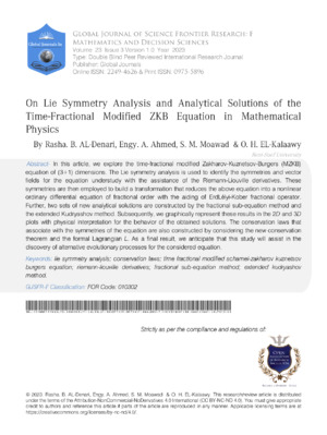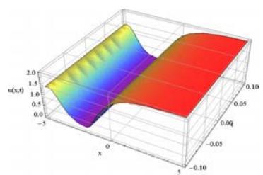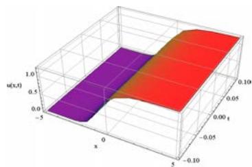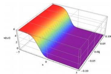The following figures show the 3D and 2D plots for the solution Eq. (31):  (a) $\alpha = 0.6$  (b) $\alpha = 0.7$  (c) $\alpha = 0.9$ Figure 1: The 3D double-layer solution (31). (a) The solution at $\alpha = 0.6$ with the parameters $\lambda = 0.4$, $\delta = -0.5$, $\kappa_{1} = 0.6$, $\kappa_{2} = 0.3$ (b) The solution at $\alpha = 0.7$ with the same parameters. (c) The solution at $\alpha = 0.9$ with the same parameters.  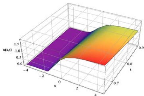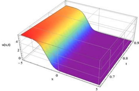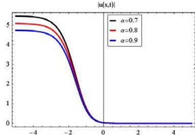(a)  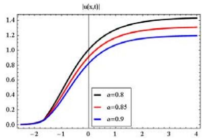(b) Figure 2: The effect of $\alpha$ on the analytical solution (36) (a) The 3D plot at a fixed time $t = 0.6$ and $0.65 \leq \alpha \leq 0.9$ with the parameters $\lambda = 0.4$, $\delta = -0.5$, $\kappa_{1} = 0.6$, $\kappa_{2} = 0.3$. (b) The 2D plot at $\alpha = 0.8$, 0.85, 0.9 and the same values of the others parameters. ## V. THE METHODOLOGY OF THE EXTENDED KUDRYASHOV METHOD We briefly display the main steps of the extended Kudryashov method [46, 47] to construct analytical solutions for Eq. (1) as below. Step 1: Consider a non-linear FODE Eq.(28) with the same traveling wave transformation as section 4 and assume that the solution of Eq.(28) can be expressed as follows: $$ q (\xi) = \sum_ {i = 0} ^ {M} B _ {i} \varphi^ {i}, \tag {37} $$ where $a_{i}$, $i = 0,1,2,\ldots,n$ are constants to be determined, and $\varphi = \varphi (\xi)$ satisfies the following equation: $$ \varphi^ {\prime} (\xi) = \varphi (\xi) ^ {3} - \varphi (\xi), \quad \text {s i n c e} \varphi (\xi) = \frac {\pm 1}{\sqrt {1 \pm e ^ {2 \xi}}} \tag {38} $$ Step 2: Determining the value of the positive integer $M$ by balancing the highest order derivatives with the nonlinear terms which appear in Eq.(28) by using the relation $M = \frac{2(s - rp)}{r - l - 1}$ since, $(q^{(p)}(\xi,\varphi))^r$ and $q^{l}(\xi,\varphi)q^{(s)}(\xi)$ are the balanced terms. Step 3: Substituting Eq.(37) into Eq.(28) and using Eq.(38), collecting all terms with the same order of $\varphi (\xi)$ together to zero yields a set of algebraic equations. Solving the equations system and using Eq.(38) to construct a variety of analytical solutions for Eq.(28). ### a) Extended Kudryashov method for Eq. (1) In this section, we apply the extended Kudryashov method method for Eq. (33) which is considered a reduced form of Eq. (1) and according to the previous analysis of the considered method. We have the following solution $$ v (\xi) = B _ {0} + B _ {1} \varphi (\xi) + B _ {2} \varphi^ {2} (\xi), \tag {39} $$ substituting Eq. (39) along with (38) into (33) and equate all the coefficients $(\varphi(\eta))^i$ by zero to get a system of algebraic equations. Solving this system with the aid of the Mathematica program we have $$ \text {C a s e 1 :} B _ {0} = 0, \quad B _ {1} = 0, \quad B _ {2} = \frac {3 \lambda^ {\alpha}}{2 \kappa_ {1}}, \quad \kappa_ {3} = - \frac {\kappa_ {2}}{2}, \quad \kappa_ {4} = - \frac {\lambda^ {\alpha}}{4}, $$ then, Eq. (1) has the below solutions $$ q _ {1 1} (\xi) = \frac {9 \lambda^ {2 \alpha}}{1 6 \kappa_ {1} ^ {2}} e ^ {- 2 \xi} s e c h ^ {2} (\xi), $$ $$ q _ {1 2} (\xi) = \frac {9 \lambda^ {2 \alpha}}{1 6 \kappa_ {1} ^ {2}} e ^ {- 2 \xi} c s c h ^ {2} (\xi). \tag {40} $$ $$ \text {C a s e 2 :} \quad B _ {0} = \frac {3 \lambda^ {\alpha}}{2 \kappa_ {1}}, \quad B _ {1} = 0, \quad B _ {2} = - \frac {3 \lambda^ {\alpha}}{2 \kappa_ {1}}, \quad \kappa_ {3} = - \frac {\kappa_ {2}}{2}, \quad \kappa_ {4} = \frac {\lambda^ {\alpha}}{4}, $$ thus, we have the next solutions for Eq. (1) which is presented as follows $$ q _ {2 1} (\xi) = \frac {9 \lambda^ {4 \alpha}}{1 6 \kappa_ {1} ^ {2}} \left(1 - \frac {1}{2} e ^ {- 2 \xi} \operatorname {s e c h} (\xi)\right) ^ {2}, $$ $$ q _ {2 2} (\xi) = \frac {9 \lambda^ {4 \alpha}}{1 6 \kappa_ {1} ^ {2}} \left(1 - \frac {1}{2} e ^ {- 2 \xi} c s c h (\xi)\right) ^ {2}. \tag {41} $$ where $\xi = x + y + z - \lambda t$ The 3D and 2D plots for the solution Eq. 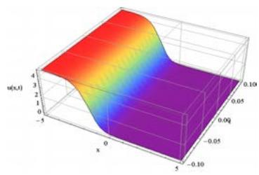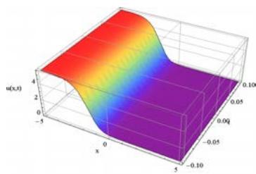(41) are plotted in the following Figures:  (a) $\alpha = 0.6$  (b) $\alpha = 0.7$  (c) $\alpha = 0.9$ Figure 3: The 3D double-layer solution (41). (a) The solution at $\alpha = 0.6$ with the parameters $\lambda = 0.7$ $\kappa_{1} = 0.5$ $\kappa_{2} = 0.3$ (b) The solution at $\alpha = 0.7$ with the same parameters. (c) The solution at $\alpha = 0.9$ with the same parameters.  (a)  (b) Figure 4: The effect of $\alpha$ on the analytical solution (41) (a) The 3D plot at a fixed time $t = 0.3$ and $0.65 \leq \alpha \leq 0.9$ with the parameters $\lambda = 0.7$, $\kappa_{1} = 0.5$, $\kappa_{2} = 0.3$. (b) The 2D plot at $\alpha = 0.7$, 0.8, 0.9 and the same values of the others parameters. ## VI. CONSERVATION LAWS FOR EQ.(1) In this section, the conservation laws of the time fractional MZKB equation (1) were derived, based on the formal lagrangian and Lie point symmetries as described in the following explanation: Consider a vector $C = (C^t,C^x,C^y,C^z)$ admits the following conservation equation $$ \left[ D _ {t} \left(C ^ {t}\right) + D _ {x} \left(C ^ {x}\right) + D _ {y} \left(C ^ {y}\right) + D _ {z} \left(C ^ {z}\right) \right] _ {E q. (1)} = 0, \tag {42} $$ where $C^t = C^t(x, y, z, t, u, \ldots)$, $C^x = C^x(x, y, z, t, u, \ldots)$, $C^y = C^y(x, y, z, t, u, \ldots)$, and $C^z = C^z(x, y, z, t, u, \ldots)$ are called the conserved vectors for Eq. (1). According to the new conservation theorem for Ibragimov [37], the formal Lagrangian for Eq. (1) can be given by $$ L = \omega ((x, y, z, t) [ \partial_ {t} ^ {\alpha} q + \kappa_ {1} \sqrt {q} q _ {x} + \kappa_ {2} q _ {x x x} + \kappa_ {3} (q _ {x y y} + q _ {x z z}) + \kappa_ {4} q _ {x x} ] = 0, \tag {43} $$ here $\omega((x, y, z, t)$ is a new dependent variable. Depending on the definition of the Lagrangian, we get an action integral as follows $$ \int_ {0} ^ {t} \int_ {\Omega_ {1}} \int_ {\Omega_ {2}} \int_ {\Omega_ {3}} L (x, y, z, t, q, \omega , D _ {t} ^ {\alpha}, q _ {x}, q _ {x x x}, q _ {x y y}, q _ {x z z}, q _ {x x}) d x d y d z d t. $$ The Euler-Lagrange operator is defined as $$ \frac {\delta}{\delta q} = \frac {\partial}{\partial q} + \left(D _ {t} ^ {\alpha}\right) ^ {*} \frac {\partial}{\partial D _ {t} ^ {\alpha} q} - D _ {x} \frac {\partial}{\partial q _ {x}} + D _ {x} ^ {2} \frac {\partial}{\partial q _ {x x}} - D _ {x} ^ {3} \frac {\partial}{\partial q _ {x x x}} - D _ {x} D _ {y} ^ {2} \frac {\partial}{\partial q _ {x y y}} - D _ {x} D _ {z} ^ {2} \frac {\partial}{\partial q _ {x z z}} $$ where $(D_t^\alpha)^*$ denotes to the adjoint operator of $D_{t}^{\alpha}$, and the adjoint equation to the nonlinear by means of the Euler-Lagrange equation is given by $$ \frac {\delta L}{\delta u} = 0. $$ Adjoint operator $(D_t^\alpha)^*$ for R-L is defined by $$ \left(D _ {t} ^ {\alpha}\right) ^ {*} = (- 1) ^ {n} I _ {T} ^ {n - \alpha} \left(D _ {t} ^ {n}\right) \equiv_ {t} ^ {C} D _ {T} ^ {\alpha}, $$ where $I_T^{n - \alpha}$ is the right-sided operator of fractional integration of order $n - \alpha$ that is defined by $$ I _ {T} ^ {n - \alpha} f (t, x) = \frac {1}{\Gamma (n - \alpha)} \int_ {t} ^ {T} (\tau - t) ^ {n - \alpha - 1} f (\tau , x) d \tau . $$ Considering the case of one dependent variable $u(x,y,z,t)$ with four independent variables $x, y, z, t$, we get $$ \bar {X} + D _ {t} (\tau) I + D _ {x} (\xi) I + D _ {y} (\zeta) I + D _ {z} (\nu) I = W \frac {\delta}{\delta u} + D _ {t} (C ^ {t}) + D _ {x} (C ^ {x}) + D _ {y} (C ^ {y}) + D _ {z} (C ^ {z}), $$ where $\bar{X}$ is defined by $$ \bar {X} = \tau \frac {\partial}{\partial t} + \xi \frac {\partial}{\partial x} + \zeta \frac {\partial}{\partial y} + \nu \frac {\partial}{\partial z} + \eta \frac {\partial}{\partial u} + \eta_ {\alpha} ^ {0} \frac {\partial}{\partial D _ {t} ^ {\alpha} u} + \eta^ {x} \frac {\partial}{\partial u _ {x}} + \eta^ {x x} \frac {\partial}{\partial u _ {x x}} + \eta^ {x x x} \frac {\partial}{\partial u _ {x x x}} + \eta^ {x y y} \frac {\partial}{\partial u _ {x y y}} + \eta^ {x z z} \frac {\partial}{\partial u _ {x z z}}, $$ and the Lie characteristic function $W$ for case 1 and 2 in the subsection 3.1 is defined as $$ W = \eta - \tau u _ {t} - \xi u _ {x} - \zeta u _ {y} - \nu u _ {z}, $$ where $W$ can be expanded to $$ W _ {1} = - \frac {\partial}{\partial t}, \quad W _ {2} = - \frac {\partial}{\partial x}, \quad W _ {3} = - \frac {\partial}{\partial y}, \quad W _ {4} = - \frac {\partial}{\partial z}, \tag {44} $$ $$ W _ {5} = - \frac {3 t}{2 \alpha} \frac {\partial}{\partial t} - \frac {x}{2} \frac {\partial}{\partial x} - \frac {y}{2} \frac {\partial}{\partial y} - \frac {z}{2} \frac {\partial}{\partial z} - 2 q \frac {\partial}{\partial q}. $$ For the R-L time-fractional derivative, the density component $C^t$ of conservation law is defined as: $$ C ^ {t} = \tau L + \sum_ {k = 0} ^ {n - 1} (- 1) ^ {k} _ {0} D _ {t} ^ {\alpha - 1 - k} \left(W _ {m}\right) D _ {t} ^ {k} \frac {\partial L}{\partial {} _ {0} D _ {t} ^ {\alpha} q} - (- 1) ^ {n} J \left(W _ {m}, D _ {t} ^ {n} \frac {\partial L}{\partial {} _ {0} D _ {t} ^ {\alpha} q}\right), \tag {45} $$ where the operator $J(\cdot)$ defined by $$ J (f, g) = \frac {1}{\Gamma (n - \alpha)} \int_ {0} ^ {t} \int_ {t} ^ {T} \frac {f (\tau , x , y , z) g (\mu , x , y , z)}{(\mu - \tau) ^ {\alpha + 1 - n}} d \mu d \tau , $$ and the other (flux) components are defined as $$ \begin{array}{l} C ^ {i} = \xi^ {i} L + W _ {m} \left[ \frac {\partial L}{\partial q _ {i} ^ {m}} - D _ {j} \left(\frac {\partial L}{\partial q _ {i j} ^ {m}}\right) + D _ {j} D _ {k} \quad \frac {\partial L}{\partial q _ {i j k} ^ {m}} - \dots\right) \bigg ] + D _ {j} (W _ {m}) \left[ \frac {\partial L}{\partial q _ {i j} ^ {m}} - D _ {k} \quad \frac {\partial L}{\partial q _ {i j k} ^ {m}}\right) + \dots \bigg ] \\+ D _ {j} D _ {k} \left(W _ {m}\right) \left. \frac {\partial L}{\partial q _ {i j k} ^ {m}} - \dots\right) + \dots , \tag {46} \\\end{array} $$ where $\xi^1 = \xi$, $\xi^2 = \zeta$, $\xi^3 = \nu$ and $m = 1,2, \ldots, 5$. Now by using Eq. (44) with the help of Eqs. (45) and (46), we obtain the components of conservation laws for the time-fractional MZKB equation as the follows Case 1: When $\kappa_4 = 0$ we have the following subcases according to the vector fields Eq. (14) Case 1.1: $W_{1} = -q_{x}$ where $\xi^{x} = 1$, $\xi^{t} = 0$, $\xi^{y} = 0$, $\xi^{z} = 0$ and $\eta = 0$ we get $$ C _ {1} ^ {t} = \omega_ {0} D _ {t} ^ {\alpha - 1} (- q _ {x}) \frac {\partial L}{\partial {} _ {0} D _ {t} ^ {\alpha} q} - J \left(- q _ {x}, D _ {t} ^ {n} \frac {\partial L}{\partial {} _ {0} D _ {t} ^ {\alpha} q}\right) = - \omega D _ {t} ^ {\alpha} (q _ {x}) - q _ {x} D _ {t} ^ {\alpha} (\omega), $$ $$ \begin{array}{l} C _ {1} ^ {x} = \omega \left[ D _ {t} ^ {\alpha} q + \kappa_ {1} \sqrt {q} q _ {x} + \frac {\kappa_ {3}}{3} (q _ {y x y} + q _ {y y x} + q _ {z x z} + q _ {z z x}) \right] - q _ {x} \left[ \kappa_ {2} \omega_ {x x} + \frac {\kappa_ {3}}{3} (\omega_ {y y} + \omega_ {z z}) \right] \\+ \kappa_ {2} q _ {x x} \omega_ {x} + \frac {\kappa_ {3}}{3} \left(q _ {x y} \omega_ {y} + q _ {x z} \omega_ {z}\right), \\\end{array} $$ $$ C _ {1} ^ {y} = - \frac {\kappa_ {3}}{3} q _ {x} [ \omega_ {x y} + \omega_ {y x} ] + \frac {\kappa_ {3}}{3} (q _ {x x} \omega_ {y} + q _ {x y} \omega_ {x}) - \frac {\kappa_ {3}}{3} \omega (q _ {x y x} + q _ {y x x}), $$ $$ C _ {1} ^ {z} = - \frac {\kappa_ {3}}{3} q _ {x} [ \omega_ {x z} + \omega_ {z x} ] + \frac {\kappa_ {3}}{3} (q _ {x x} \omega_ {z} + q _ {x z} \omega_ {x}) - \frac {\kappa_ {3}}{3} \omega (q _ {x z x} + q _ {z x x}), $$ Case 1.2: $W_{2} = -q_{t}$ where $\xi^{x} = 0$, $\xi^{t} = 1$, $\xi^{y} = 0$, $\xi^{z} = 0$ and $\eta = 0$ we obtain $$ \begin{array}{l} C _ {2} ^ {t} = \omega L \omega_ {0} D _ {t} ^ {\alpha - 1} (- q _ {t}) \frac {\partial L}{\partial {} _ {0} D _ {t} ^ {\alpha} q} - J \left(- q _ {t}, D _ {t} ^ {n} \frac {\partial L}{\partial {} _ {0} D _ {t} ^ {\alpha} q}\right) \\= \omega \left[ D _ {t} ^ {\alpha} q + \kappa_ {1} \sqrt {q} q _ {x} + \frac {\kappa_ {3}}{3} (q _ {y x y} + q _ {y y x} + q _ {z x z} + q _ {z z x}) \right] - \omega D _ {t} ^ {\alpha} (q _ {t}) - q _ {t} D _ {t} ^ {\alpha} (\omega), \\\end{array} $$ $$ \begin{array}{l} C _ {2} ^ {x} = - q _ {t} \Big [ \kappa_ {1} \omega \sqrt {q} - \kappa_ {4} \omega_ {x} + \kappa_ {2} \omega_ {x x} + \frac {\kappa_ {3}}{3} (\omega_ {y y} + \omega_ {z z}) \Big ] - q _ {x t} \big [ - \kappa_ {2} \omega_ {x} \big ] + \frac {\kappa_ {3}}{3} (q _ {y t} \omega_ {y} + q _ {z t} \omega_ {z}) \\- \kappa_ {2} \omega q _ {x x t} - \frac {\kappa_ {3}}{3} \omega \left(q _ {y y t} + q _ {z z t}\right), \\\end{array} $$ $$ C _ {2} ^ {y} = - \frac {\kappa_ {3}}{3} q _ {t} \left[ \omega_ {x y} + \omega_ {y x} \right] + \frac {\kappa_ {3}}{3} \left(q _ {x t} \omega_ {y} + q _ {y t} \omega_ {x}\right) - \frac {\kappa_ {3}}{3} \omega \left(q _ {x y t} + q _ {y x t}\right), $$ $$ C _ {2} ^ {z} = - \frac {\kappa_ {3}}{3} q _ {t} [ \omega_ {x z} + \omega_ {z x} ] + \frac {\kappa_ {3}}{3} (q _ {x t} \omega_ {z} + q _ {z t} \omega_ {x}) - \frac {\kappa_ {3}}{3} \omega (q _ {x z t} + q _ {z x t}) $$ Case 1.3: $W_{3} = -q_{y}$ where $\xi^{x} = 0$, $\xi^{t} = 0$, $\xi^{y} = 1$, $\xi^{z} = 0$ and $\eta = 0$ we have $$ C _ {3} ^ {t} = \omega_ {0} D _ {t} ^ {\alpha - 1} (- q _ {y}) \frac {\partial L}{\partial {} _ {0} D _ {t} ^ {\alpha} q} - J \left(- q _ {y}, D _ {t} ^ {n} \frac {\partial L}{\partial {} _ {0} D _ {t} ^ {\alpha} q}\right) = - \omega D _ {t} ^ {\alpha} (q _ {y}) - q _ {y} D _ {t} ^ {\alpha} (\omega), $$ $$ \begin{array}{l} C _ {3} ^ {x} = - q _ {y} \Big [ \kappa_ {1} \omega \sqrt {q} - \kappa_ {4} \omega_ {x} + \kappa_ {2} \omega_ {x x} + \frac {\kappa_ {3}}{3} (\omega_ {y y} + \omega_ {z z}) \Big ] - q _ {x y} [ - \kappa_ {2} \omega_ {x} ] + \frac {\kappa_ {3}}{3} (q _ {y y} \omega_ {y} + q _ {y z} \omega_ {z}) \\- \kappa_ {2} \omega q _ {x x y} - \frac {\kappa_ {3}}{3} \omega \left(q _ {y y y} + q _ {z z y}\right), \\\end{array} $$ $$ \begin{array}{l} C _ {3} ^ {y} = \omega \left[ D _ {t} ^ {\alpha} q + a \sqrt {q} q _ {x} + \frac {\kappa_ {3}}{3} (q _ {y x y} + q _ {y y x} + q _ {z x z} + q _ {z z x}) \right] - \frac {\kappa_ {3}}{3} q _ {y} [ \omega_ {x y} + \omega_ {y x} ] \\+ \frac {\kappa_ {3}}{3} \left(q _ {x y} \omega_ {y} + q _ {y y} \omega_ {x}\right) - \frac {\kappa_ {3}}{3} \omega \left(q _ {x y y} + q _ {y x y}\right), \\\end{array} $$ $$ C _ {3} ^ {z} = - \frac {\kappa_ {3}}{3} q _ {y} [ \omega_ {x z} + \omega_ {z x} ] + \frac {\kappa_ {3}}{3} (q _ {x y} \omega_ {z} + q _ {y z} \omega_ {x}) - \frac {\kappa_ {3}}{3} \omega (q _ {x z y} + q _ {z x y}), $$ Case 1.4: $W_{4} = -q_{z}$ where $\xi^{x} = 0$, $\xi^{t} = 0$, $\xi^{y} = 0$, $\xi^{z} = 1$ and $\eta = 0$ we obtain $$ C _ {4} ^ {t} = \omega_ {0} D _ {t} ^ {\alpha - 1} (- q _ {z}) \frac {\partial L}{\partial_ {0} D _ {t} ^ {\alpha} q} - J \left(- q _ {z}, D _ {t} ^ {n} \frac {\partial L}{\partial_ {0} D _ {t} ^ {\alpha} q}\right) = - \omega D _ {t} ^ {\alpha} (q _ {z}) - q _ {z} D _ {t} ^ {\alpha} (\omega), $$ $$ \begin{array}{l} C _ {4} ^ {x} = - q _ {z} \left[ \kappa_ {1} \omega \sqrt {q} - \kappa_ {4} \omega_ {x} + \kappa_ {2} \omega_ {x x} + \frac {\kappa_ {3}}{3} (\omega_ {y y} + \omega_ {z z}) \right] - q _ {x y} [ - \kappa_ {2} \omega_ {x} ] + \frac {\kappa_ {3}}{3} (q _ {y y} \omega_ {y} + q _ {y z} \omega_ {z}) \\- \kappa_ {2} \omega q _ {x x y} - \frac {\kappa_ {3}}{3} \omega (q _ {y y y} + q _ {z z y}), \\\end{array} $$ $$ C _ {4} ^ {y} = - \frac {\kappa_ {3}}{3} q _ {y} \left[ \omega_ {x y} + \omega_ {y x} \right] + \frac {\kappa_ {3}}{3} \left(q _ {x y} \omega_ {y} + q _ {y y} \omega_ {x}\right) - \frac {\kappa_ {3}}{3} \omega \left(q _ {x y y} + q _ {y x y}\right), $$ $$ \begin{array}{l} C _ {4} ^ {z} = \omega \left[ D _ {t} ^ {\alpha} q + a \sqrt {q} q _ {x} + \frac {\kappa_ {3}}{3} (q _ {y x y} + q _ {y y x} + q _ {z x z} + q _ {z z x}) \right] \\- \frac {\kappa_ {3}}{3} q _ {y} \left[ \omega_ {x z} + \omega_ {z x} \right] + \frac {\kappa_ {3}}{3} \left(q _ {x y} \omega_ {z} + q _ {y z} \omega_ {x}\right) - \frac {\kappa_ {3}}{3} \omega \left(q _ {x z y} + q _ {z x y}\right). \\\end{array} $$ Case 1.5: $W_{5} = -2q - \frac{3t}{2\alpha}\frac{\partial}{\partial t} -\frac{x}{2}\frac{\partial}{\partial x} -\frac{y}{2}\frac{\partial}{\partial y} -\frac{z}{2}\frac{\partial}{\partial z}$ then $$ \begin{array}{l} C _ {5} ^ {t} = \omega_ {0} D _ {t} ^ {\alpha - 1} (- q _ {z}) \frac {\partial L}{\partial {} _ {0} D _ {t} ^ {\alpha} q} - J \left(- q _ {z}, D _ {t} ^ {n} \frac {\partial L}{\partial {} _ {0} D _ {t} ^ {\alpha} q}\right) \\= \frac {3 t}{2 \alpha} \omega \left[ D _ {t} ^ {\alpha} q + \kappa_ {1} \sqrt {q} q _ {x} + \frac {\kappa_ {3}}{3} \left(q _ {y x y} + q _ {y y x} + q _ {z x z} + q _ {z z x}\right) \right] \\- \omega D _ {t} ^ {\alpha} \left(2 q + \frac {3 t}{2 \alpha} \frac {\partial}{\partial t} + \frac {x}{2} \frac {\partial}{\partial x} + \frac {y}{2} \frac {\partial}{\partial y} + \frac {z}{2} \frac {\partial}{\partial z}\right) + \left(2 q + \frac {3 t}{2 \alpha} \frac {\partial}{\partial t} + \frac {x}{2} \frac {\partial}{\partial x} + \frac {y}{2} \frac {\partial}{\partial y} + \frac {z}{2} \frac {\partial}{\partial z}\right) D _ {t} ^ {\alpha} (\omega), \\\end{array} $$ $$ \begin{array}{l} C _ {5} ^ {x} = \frac {x}{2} \omega \left[ D _ {t} ^ {\alpha} q + \kappa_ {1} \sqrt {q} q _ {x} + \frac {\kappa_ {3}}{3} \left(q _ {y x y} + q _ {y y x} + q _ {z x z} + q _ {z z x}\right) \right] \\\left. - \left(2 q + \frac {3 t}{2 \alpha} \frac {\partial}{\partial t} + \frac {x}{2} \frac {\partial}{\partial x} + \frac {y}{2} \frac {\partial}{\partial y} + \frac {z}{2} \frac {\partial}{\partial z}\right) \left[ \kappa_ {2} \omega_ {x x} + \frac {\kappa_ {3}}{3} (\omega_ {y y} + \omega_ {z z}) \right] \right. \\+ \kappa_ {2} \omega_ {x} \frac {\partial}{\partial x} \left(2 q + \frac {3 t}{2 \alpha} \frac {\partial}{\partial t} + \frac {x}{2} \frac {\partial}{\partial x} + \frac {y}{2} \frac {\partial}{\partial y} + \frac {z}{2} \frac {\partial}{\partial z}\right) + \frac {\kappa_ {3}}{3} \left(\omega_ {y} \frac {\partial}{\partial y} \left(2 q + \frac {3 t}{2 \alpha} \frac {\partial}{\partial t} + \frac {x}{2} \frac {\partial}{\partial x} + \frac {y}{2} \frac {\partial}{\partial y} + \frac {z}{2} \frac {\partial}{\partial z}\right) \right. \\\left. + \omega_ {z} \frac {\partial}{\partial z} \left(2 q + \frac {3 t}{2 \alpha} \frac {\partial}{\partial t} + \frac {x}{2} \frac {\partial}{\partial x} + \frac {y}{2} \frac {\partial}{\partial y} + \frac {z}{2} \frac {\partial}{\partial z}\right)\right), \\\end{array} $$ $$ \begin{array}{l} C _ {5} ^ {y} = \frac {y}{2} \omega \Big [ D _ {t} ^ {\alpha} q + a \sqrt {q} q _ {x} + \frac {\kappa_ {3}}{3} (q _ {y x y} + q _ {y y x} + q _ {z x z} + q _ {z z x}) \Big ] - \frac {\kappa_ {3}}{3} \left(2 q + \frac {3 t}{2 \alpha} \frac {\partial}{\partial t} + \frac {x}{2} \frac {\partial}{\partial x} + \frac {y}{2} \frac {\partial}{\partial y} + \frac {z}{2} \frac {\partial}{\partial z}\right) [ \omega_ {x y} + \omega_ {y x} ] \\+ \frac {\kappa_ {3}}{3} \left(\omega_ {y} \frac {\partial}{\partial x} \left(2 q + \frac {3 t}{2 \alpha} \frac {\partial}{\partial t} + \frac {x}{2} \frac {\partial}{\partial x} + \frac {y}{2} \frac {\partial}{\partial y} + \frac {z}{2} \frac {\partial}{\partial z}\right) + \omega_ {x} \frac {\partial}{\partial y} \left(2 q + \frac {3 t}{2 \alpha} \frac {\partial}{\partial t} + \frac {x}{2} \frac {\partial}{\partial x} + \frac {y}{2} \frac {\partial}{\partial y} + \frac {z}{2} \frac {\partial}{\partial z}\right)\right) \\- \frac {\kappa_ {3}}{3} \omega \frac {\partial}{\partial x y} \left(2 q + \frac {3 t}{2 \alpha} \frac {\partial}{\partial t} + \frac {x}{2} \frac {\partial}{\partial x} + \frac {y}{2} \frac {\partial}{\partial y} + \frac {z}{2} \frac {\partial}{\partial z}\right), \\\end{array} $$ $$ \begin{array}{l} C _ {5} ^ {z} = \frac {z}{2} \omega \Big [ D _ {t} ^ {\alpha} q + a \sqrt {q} q _ {x} + \frac {\kappa_ {3}}{3} (q _ {y x y} + q _ {y y x} + q _ {z x z} + q _ {z z x}) \Big ] - \frac {\kappa_ {3}}{3} \left(2 q + \frac {3 t}{2 \alpha} \frac {\partial}{\partial t} + \frac {x}{2} \frac {\partial}{\partial x} + \frac {y}{2} \frac {\partial}{\partial y} + \frac {z}{2} \frac {\partial}{\partial z}\right) [ \omega_ {x z} + \omega_ {z x} ] \\+ \frac {\kappa_ {3}}{3} \left(\omega_ {y} \frac {\partial}{\partial x} \left(2 q + \frac {3 t}{2 \alpha} \frac {\partial}{\partial t} + \frac {x}{2} \frac {\partial}{\partial x} + \frac {y}{2} \frac {\partial}{\partial y} + \frac {z}{2} \frac {\partial}{\partial z}\right) + \omega_ {x} \frac {\partial}{\partial z} \left(2 q + \frac {3 t}{2 \alpha} \frac {\partial}{\partial t} + \frac {x}{2} \frac {\partial}{\partial x} + \frac {y}{2} \frac {\partial}{\partial y} + \frac {z}{2} \frac {\partial}{\partial z}\right)\right) \\- \frac {\kappa_ {3}}{3} \omega \frac {\partial}{\partial x z} \left(2 q + \frac {3 t}{2 \alpha} \frac {\partial}{\partial t} + \frac {x}{2} \frac {\partial}{\partial x} + \frac {y}{2} \frac {\partial}{\partial y} + \frac {z}{2} \frac {\partial}{\partial z}\right). \\\end{array} $$ Case 2: When $\kappa_4 \neq 0$ we have the following subcases according to the vector fields Eq. (14) Case 2.1: $W_{1} = -q_{x}$ where $\xi^{x} = 1$, $\xi^{t} = 0$, $\xi^{y} = 0$, $\xi^{z} = 0$ and $\eta = 0$ we get $$ C _ {1} ^ {t} = \omega_ {0} D _ {t} ^ {\alpha - 1} (- q _ {x}) \frac {\partial L}{\partial_ {0} D _ {t} ^ {\alpha} q} - J \left(- q _ {x}, D _ {t} ^ {n} \frac {\partial L}{\partial_ {0} D _ {t} ^ {\alpha} q}\right) = - \omega D _ {t} ^ {\alpha} (q _ {x}) - q _ {x} D _ {t} ^ {\alpha} (\omega), $$ $$ \begin{array}{l} C _ {1} ^ {x} = \omega \left[ D _ {t} ^ {\alpha} q + \kappa_ {1} \sqrt {q} q _ {x} + \frac {\kappa_ {3}}{3} \left(q _ {y x y} + q _ {y y x} + q _ {z x z} + q _ {z z x}\right) \right] - q _ {x} \left[ - \kappa_ {4} \omega_ {x} + \kappa_ {2} \omega_ {x x} + \frac {\kappa_ {3}}{3} \left(\omega_ {y y} + \omega_ {z z} \right. \right] \\+ \kappa_ {2} q _ {x x} \omega_ {x} + \frac {\kappa_ {3}}{3} \left(q _ {x y} \omega_ {y} + q _ {x z} \omega_ {z}\right), \\\end{array} $$ $$ C _ {1} ^ {y} = - \frac {\kappa_ {3}}{3} q _ {x} \left[ \omega_ {x y} + \omega_ {y x} \right] + \frac {\kappa_ {3}}{3} \left(q _ {x x} \omega_ {y} + q _ {x y} \omega_ {x}\right) - \frac {\kappa_ {3}}{3} \omega \left(q _ {x y x} + q _ {y x x}\right), $$ $$ C _ {1} ^ {z} = - \frac {\kappa_ {3}}{3} q _ {x} \left[ \omega_ {x z} + \omega_ {z x} \right] + \frac {\kappa_ {3}}{3} \left(q _ {x x} \omega_ {z} + q _ {x z} \omega_ {x}\right) - \frac {\kappa_ {3}}{3} \omega \left(q _ {x z x} + q _ {z x x}\right), $$ Case 2.2: $W_{2} = -q_{t}$ where $\xi^{x} = 0$, $\xi^{t} = 1$, $\xi^{y} = 0$, $\xi^{z} = 0$ and $\eta = 0$ we obtain $$ \begin{array}{l} C _ {2} ^ {t} = \omega L \omega_ {0} D _ {t} ^ {\alpha - 1} (- q _ {t}) \frac {\partial L}{\partial {} _ {0} D _ {t} ^ {\alpha} q} - J \left(- q _ {t}, D _ {t} ^ {n} \frac {\partial L}{\partial {} _ {0} D _ {t} ^ {\alpha} q}\right) \\= \omega \left[ D _ {t} ^ {\alpha} q + \kappa_ {1} \sqrt {q} q _ {x} + \frac {\kappa_ {3}}{3} (q _ {y x y} + q _ {y y x} + q _ {z x z} + q _ {z z x}) + \kappa_ {4} q _ {x x} \right] - \omega D _ {t} ^ {\alpha} (q _ {t}) - q _ {t} D _ {t} ^ {\alpha} (\omega), \\\end{array} $$ $$ \begin{array}{l} C _ {2} ^ {x} = - q _ {t} \Big [ \kappa_ {1} \omega \sqrt {q} - \kappa_ {4} \omega_ {x} + \kappa_ {2} \omega_ {x x} + \frac {\kappa_ {3}}{3} (\omega_ {y y} + \omega_ {z z} \Big ] - q _ {x t} [ \kappa_ {4} \omega_ {x} - \kappa_ {2} \omega_ {x} ] + \frac {\kappa_ {3}}{3} (q _ {y t} \omega_ {y} + q _ {z t} \omega_ {z}) \\- \kappa_ {2} \omega q _ {x x t} - \frac {\kappa_ {3}}{3} \omega (q _ {y y t} + q _ {z z t}), \\\end{array} $$ $$ C _ {2} ^ {y} = - \frac {\kappa_ {3}}{3} q _ {t} [ \omega_ {x y} + \omega_ {y x} ] + \frac {\kappa_ {3}}{3} (q _ {x t} \omega_ {y} + q _ {y t} \omega_ {x}) - \frac {\kappa_ {3}}{3} \omega (q _ {x y t} + q _ {y x t}), $$ $$ C _ {2} ^ {z} = - \frac {\kappa_ {3}}{3} q _ {t} \left[ \omega_ {x z} + \omega_ {z x} \right] + \frac {\kappa_ {3}}{3} \left(q _ {x t} \omega_ {z} + q _ {z t} \omega_ {x}\right) - \frac {\kappa_ {3}}{3} \omega \left(q _ {x z t} + q _ {z x t}\right) $$ Case 2.3: $W_{3} = -u_{y}$ where $\xi^{x} = 0$, $\xi^{t} = 0$, $\xi^{y} = 1$, $\xi^{z} = 0$ and $\eta = 0$ we have $$ C _ {3} ^ {t} = \omega_ {0} D _ {t} ^ {\alpha - 1} (- q _ {y}) \frac {\partial L}{\partial_ {0} D _ {t} ^ {\alpha} q} - J \left(- q _ {y}, D _ {t} ^ {n} \frac {\partial L}{\partial_ {0} D _ {t} ^ {\alpha} q}\right) = - \omega D _ {t} ^ {\alpha} (q _ {y}) - q _ {y} D _ {t} ^ {\alpha} (\omega), $$ $$ \begin{array}{l} C _ {3} ^ {x} = - q _ {y} \left[ \kappa_ {1} \omega \sqrt {q} - \kappa_ {4} \omega_ {x} + \kappa_ {2} \omega_ {x x} + \frac {\kappa_ {3}}{3} (\omega_ {y y} + \omega_ {z z}) \right] - q _ {x y} \left[ \kappa_ {4} \omega_ {x} - \kappa_ {2} \omega_ {x} \right] + \frac {\kappa_ {3}}{3} (q _ {y y} \omega_ {y} + q _ {y z} \omega_ {z}) \\- \kappa_ {2} \omega q _ {x x y} - \frac {\kappa_ {3}}{3} \omega (q _ {y y y} + q _ {z z y}), \\\end{array} $$ $$ \begin{array}{l} C _ {3} ^ {y} = \omega \left[ D _ {t} ^ {\alpha} q + a \sqrt {q} q _ {x} + \frac {\kappa_ {3}}{3} (q _ {y x y} + q _ {y y x} + q _ {z x z} + q _ {z z x}) + \kappa_ {4} q _ {x x} \right] - \frac {\kappa_ {3}}{3} q _ {y} [ \omega_ {x y} + \omega_ {y x} ] \\+ \frac {\kappa_ {3}}{3} (q _ {x y} \omega_ {y} + q _ {y y} \omega_ {x}) - \frac {\kappa_ {3}}{3} \omega (q _ {x y y} + q _ {y x y}), \\\end{array} $$ $$ C _ {3} ^ {z} = - \frac {\kappa_ {3}}{3} q _ {y} [ \omega_ {x z} + \omega_ {z x} ] + \frac {\kappa_ {3}}{3} (q _ {x y} \omega_ {z} + q _ {y z} \omega_ {x}) - \frac {\kappa_ {3}}{3} \omega (q _ {x z y} + q _ {z x y}), $$ Case 2.4: $W_{4} = -q_{z}$ where $\xi^{x} = 0$, $\xi^{t} = 0$, $\xi^{y} = 0$, $\xi^{z} = 0$ and $\eta = 0$ we obtain $$ C _ {4} ^ {t} = \omega_ {0} D _ {t} ^ {\alpha - 1} (- q _ {z}) \frac {\partial L}{\partial {} _ {0} D _ {t} ^ {\alpha} q} - J \left(- q _ {z}, D _ {t} ^ {n} \frac {\partial L}{\partial {} _ {0} D _ {t} ^ {\alpha} q}\right) = - \omega D _ {t} ^ {\alpha} (q _ {z}) - q _ {z} D _ {t} ^ {\alpha} (\omega), $$ $$ \begin{array}{l} C _ {4} ^ {x} = - q _ {z} \left[ \kappa_ {1} \omega \sqrt {q} - \kappa_ {4} \omega_ {x} + \kappa_ {2} \omega_ {x x} + \frac {\kappa_ {3}}{3} (\omega_ {y y} + \omega_ {z z} \right] - q _ {x y} [ \kappa_ {4} \omega_ {x} - \kappa_ {2} \omega_ {x} ] + \frac {\kappa_ {3}}{3} (q _ {y y} \omega_ {y} + q _ {y z} \omega_ {z}) \\- \kappa_ {2} \omega q _ {x x y} - \frac {\kappa_ {3}}{3} \omega (q _ {y y y} + q _ {z z y}), \\\end{array} $$ $$ \begin{array}{l} C _ {4} ^ {y} = \omega \left[ D _ {t} ^ {\alpha} q + a \sqrt {q} q _ {x} + \frac {\kappa_ {3}}{3} (q _ {y x y} + q _ {y y x} + q _ {z x z} + q _ {z z x}) + \kappa_ {4} q _ {x x} \right] - \frac {\kappa_ {3}}{3} q _ {y} [ \omega_ {x y} + \omega_ {y x} ] \\+ \frac {\kappa_ {3}}{3} (q _ {x y} \omega_ {y} + q _ {y y} \omega_ {x}) - \frac {\kappa_ {3}}{3} \omega (q _ {x y y} + q _ {y x y}), \\\end{array} $$ $$ C _ {4} ^ {z} = - \frac {\kappa_ {3}}{3} q _ {y} \left[ \omega_ {x z} + \omega_ {z x} \right] + \frac {\kappa_ {3}}{3} \left(q _ {x y} \omega_ {z} + q _ {y z} \omega_ {x}\right) - \frac {\kappa_ {3}}{3} \omega \left(q _ {x z y} + q _ {z x y}\right). $$ Remark: We have verified that all the cases satisfy the equation of conservation laws Eq. (42). ## VII. CONCLUSION In this article, we considered the time-fractional modified Zakharov-Kuznetsov-Burgers (MZKB) equation of $(3 + 1)$ dimensions. With the help of the Riemann-Liouville derivatives, the Lie symmetry analysis was successfully applied to study this equation. This analysis generated the symmetries and vector fields, which aided us in constructing the similarity reductions of the considered equation. Consequently, we constructed two sets of new analytical solutions via two powerful methods which are the fractional subequation method and extended Kudryashov method. Furthermore, to gain a better understanding of the dynamics of these solutions, we graphed the 3D and 2D plots of obtained solutions using appropriate parameters. Figure 1 described the double-layer solution (31) at $\alpha = 0.6$, 0.7, 0.9 with the parameters $\lambda = 0.4$, $\delta = -0.5$, $\kappa_{1} = 0.6$, $\kappa_{2} = 0.3$ at $-5 \leq x \leq 5$. Figure 2 showed the effect of $\alpha$ on the solution (31) at a fixed time $t = 0.6$ with $\alpha = 0.8$, 0.85, 0.9 and the parameters $\lambda = 0.4$, $\delta = -0.5$, $\kappa_{1} = 0.6$, $\kappa_{2} = 0.3$ for $-2.5 \leq x \leq 4$. Figure 3 represented the double-layer solution (41) at $\alpha = 0.6$, 0.7, 0.9 with the parameters $\lambda = 0.7$, $\kappa_{1} = 0.5$, $\kappa_{2} = 0.3$ where this Figure was traced at $-5 \leq x \leq 5$. Figure 4 was graphed by taking suitable parameters as $\lambda = 0.7$, $\kappa_{1} = 0.5$, $\kappa_{2} = 0.3$ and described the stable behavior of the solution (41) at $\alpha = 0.7$, 0.8, 0.9 for $0 \leq x \leq 5$ at a fixed time $t$ and decreases as the fractional-order $\alpha$ increases outside this interval. As a consequence, we presume that the obtained results will be more useful in explaining the physical meaning of the time fractional MZKB equation. Furthermore, we obtained four kinds of conservation laws with independent variables laying the groundwork of Lie symmetries. Finally, because of accuracy, ease of application, and relevance of the used methods in this paper, they could be generalized to many FPDEs. Data availability The authors confirm that the data supporting the findings of this study are available within the article and its supplementary materials. Funding This research work is not supported by any funding agencies. Competing interests The author has declared that no competing interests exist. Contributions The authors declare that the work was realized in collaboration with a specified responsibility for each author. All authors read and approved the final paper.

Generating HTML Viewer...

References

46 Cites in Article
Mi-Gyong Ri,Chol-Hui Yun,Myong-Hun Kim (2021). Construction of cubic spline hidden variable recurrent fractal interpolation function and its fractional calculus.
Bing Guo,Ali Raza,Kamel Al-Khaled,Sami Khan,Saadia Farid,Ye Wang,M Khan,M Malik,S Saleem (2021). Fractional-order simulations for heat and mass transfer analysis confined by elliptic inclined plate with slip effects: A comparative fractional analysis.
M Khan,M Akbar,Abd Binti,N Hamid (2021). Traveling wave solutions for space-time fractional Cahn Hilliard equation and space-time fractional symmetric regularized long-wave equation.
M S Hashemi,E Ashpazzadeh,M Moharrami,M Lakestani (2021). Fractional order Alpert multiwavelets for discretizing delay fractional differential equation of pantograph type.
X Yang (2019). General fractional derivatives: Theory, methods and applications.
D Baleanu,D Kumar (2019). Fractional Calculus and its Applications in Physics.
Xian-Min Zhang (2021). A new method for searching the integral solution of system of Riemann–Liouville fractional differential equations with non-instantaneous impulses.
Shaochun Ji,Dandan Yang (2019). Solutions to Riemann–Liouville fractional integrodifferential equations via fractional resolvents.
J Graef,C Tunc,H Sevli (2021). Razumikhin qualitative analyses of Volterra integro-fractional delay differential equation with caputo derivatives.
K Wang (2021). Variational principle and approximate solution for the generalized Burgers-Huxley equation with fractal derivative.
F He,L Li (2019). Time fractional modified KdV-type equations: Lie symmetries, exact solutions and conservation laws.
Octavian Postavaru,Antonela Toma (2021). Numerical solution of two-dimensional fractional-order partial differential equations using hybrid functions.
Muhammad Farman,Muhammad Saleem,Aqeel Ahmad,M Ahmad (2018). Analysis and numerical solution of SEIR epidemic model of measles with non-integer time fractional derivatives by using Laplace Adomian Decomposition Method.
Wenjin Li,Yanni Pang (2020). Application of Adomian decomposition method to nonlinear systems.
M A Abdelkawy,O El-Kalaawy,Al-Denari R B Biswas,A (2018). Application of fractional sub-equation method to nonlinear evolution equations.
Sheng Zhang,Hong-Qing Zhang (2011). Fractional sub-equation method and its applications to nonlinear fractional PDEs.
Elaheh Saberi,S Reza Hejazi (2018). Lie symmetry analysis, conservation laws and exact solutions of the time-fractional generalized Hirota–Satsuma coupled KdV system.
Shehu Maitama,Weidong Zhao (2019). Local fractional homotopy analysis method for solving non-differentiable problems on Cantor sets.
S Sahoo,S Saha Ray,M Abdou (2020). New exact solutions for time-fractional Kaup-Kupershmidt equation using improved (G′/G)-expansion and extended (G′/G)-expansion methods.
Muhammad Ali,M S Osman,Syed Husnine (2019). On the analytical solutions of conformable time-fractional extended Zakharov–Kuznetsov equation through ( $$G'/G^{2}$$ G ′ / G 2 )-expansion method and the modified Kudryashov method.
B Tayyan,A Sakka (2020). Lie symmetry analysis of some conformable fractional partial differential equations.
Amit Prakash,Manish Goyal,Shivangi Gupta (2019). Fractional variational iteration method for solving time-fractional Newell-Whitehead-Segel equation.
C Angstmann,B Henry (2020). Generalized fractional power series solutions for fractional differential equations.
M Alaroud (2021). Application of Laplace residual power series method for approximate solutions of fractional IVP's.
Salah Abuasad,Ishak Hashim,Samsul Abdul Karim (2019). Modified Fractional Reduced Differential Transform Method for the Solution of Multiterm Time-Fractional Diffusion Equations.
Safyan Mukhtar,Salah Abuasad,Ishak Hashim,Samsul Abdul Karim (2020). Effective Method for Solving Different Types of Nonlinear Fractional Burgers’ Equations.
Dandan Shi,Yufeng Zhang,Wenhao Liu,Jiangen Liu (2019). Some Exact Solutions and Conservation Laws of the Coupled Time-Fractional Boussinesq-Burgers System.
Baljinder Kour,Sachin Kumar (2018). Symmetry analysis, explicit power series solutions and conservation laws of the space-time fractional variant Boussinesq system.
S Kumar,B Kour,S Yao,M Inc,M Osman (2021). Invariance Analysis, Exact Solution and Conservation Laws of (2+1) Dim Fractional Kadomtsev-Petviashvili (KP) System.
Xiu-Bin Wang,Shou-Fu Tian,Chun-Yan Qin,Tian-Tian Zhang (2017). Lie symmetry analysis, conservation laws and analytical solutions of a time-fractional generalized KdV-type equation*.
Xiu-Bin Wang,Shou-Fu Tian,Chun-Yan Qin,Tian-Tian Zhang (2016). Characteristics of the breathers, rogue waves and solitary waves in a generalized (2+1)-dimensional Boussinesq equation.
Jian-Gen Liu,Xiao-Jun Yang,Yi-Ying Feng,Ping Cui (2020). On group analysis of the time fractional extended (2+1)-dimensional Zakharov–Kuznetsov equation in quantum magneto-plasmas.
Jian‐gen Liu,Xiao‐jun Yang,Yi‐ying Feng,Lu‐lu Geng (2021). Numerical solutions and conservation laws of the time fractional coupled WBK‐type system.
Jian-Gen Liu,Xiao-Jun Yang,Yi-Ying Feng,Ping Cui,Lu-Lu Geng (2021). On integrability of the higher dimensional time fractional KdV-type equation.
Jian-Gen Liu,Xiao-Jun Yang,Lu-Lu Geng,Yu-Rong Fan (2021). GROUP ANALYSIS OF THE TIME FRACTIONAL (3 + 1)-DIMENSIONAL KDV-TYPE EQUATION.
Jian-Gen Liu,Xiao-Jun Yang,Lu-Lu Geng,Yu-Rong Fan,Xian-Zhen Yan (2021). Fundamental analysis of the time fractional coupled Burgers-type equations.
Shrouk Wael,Aly Seadawy,Salah Moawad,Omar El‐kalaawy (2021). Bilinear Bäcklund transformation, <i>N</i>‐soliton, and infinite conservation laws for Lax–Kadomtsev–Petviashvili and generalized Korteweg–de Vries equations.
O El-Kalaawy (2018). Modulational instability: Conservation laws and bright soliton solution of ion-acoustic waves in electron-positron-ion-dust plasmas.
O El-Kalaawy (2017). New: Variational principle–exact solutions and conservation laws for modified ion-acoustic shock waves and double layers with electron degenerate in plasma.
El-Kalaawy O H,S Moawad,M Tharwat,Al-Denari R B (2016). Variational principle, conservation laws and exact solutions for dust ion acoustic shock waves modeling modified Burger equation.
Yi Tian,Kang-Le Wang (2020). Conservation laws for partial differential equations based on the polynomial characteristic method.
Rasha Al-Denari,R Ibrahim,M Tharwat,S M Moawad,O El-Kalaawy (2022). Similarity reduction, conservation laws, and explicit solutions for the time-fractional coupled GI equation provided with convergence analysis and numerical simulation.
O El-Kalaawy,Engy Ahmed (2018). Shock Waves, Variational Principle and Conservation Laws of a Schamel–Zakharov–Kuznetsov–Burgers Equation in a Magnetised Dust Plasma.
Idir Hadjaz,Mouloud Tribeche (2014). Alternative dust-ion acoustic waves in a magnetized charge varying dusty plasma with nonthermal electrons having a vortex-like velocity distribution.
Serife Ege (2022). Solitary Wave Solutions for Some Fractional Evolution Equations via New Kudryashov Approach.
No ethics committee approval was required for this article type.
Data Availability
Not applicable for this article.
How to Cite This Article
Rasha. B. AL-Denari. 2026. \u201cOn Lie Symmetry Analysis and Analytical Solutions of the Time-Fractional Modified ZKB Equation in Mathematical Physics\u201d. Global Journal of Science Frontier Research - F: Mathematics & Decision GJSFR-F Volume 23 (GJSFR Volume 23 Issue F3): .
Explore published articles in an immersive Augmented Reality environment. Our platform converts research papers into interactive 3D books, allowing readers to view and interact with content using AR and VR compatible devices.
Your published article is automatically converted into a realistic 3D book. Flip through pages and read research papers in a more engaging and interactive format.
In this article, we explore the time-fractional modified Zakharov-Kuznetsov-Burgers (MZKB) equation of (3+1) dimensions. The Lie symmetry analysis is used to identify the symmetries and vector fields for the equation understudy with the assistance of the Riemann-Liouville derivatives. These symmetries are then employed to build a transformation that reduces the above equation into a nonlinear ordinary differential equation of fractional order with the aiding of ErdLélyi-Kober fractional operator. Further, two sets of new analytical solutions are constructed by the fractional sub-equation method and the extended Kudryashov method. Subsequently, we graphically represent these results in the 2D and 3D plots with physical interpretation for the behavior of the obtained solutions. The conservation laws that associate with the symmetries of the equation are also constructed by considering the new conservation theorem and the formal Lagrangian L. As a final result, we anticipate that this study will assist in the discovery of alternative evolutionary processes for the considered equation.
Our website is actively being updated, and changes may occur frequently. Please clear your browser cache if needed. For feedback or error reporting, please email [email protected]
Thank you for connecting with us. We will respond to you shortly.