On the Convergence of a Single Step Third Order Method for Solving Equations

Samundra Regmi; Ioannis K. Argyros; Santhosh George; Christopher I. Argyros

I. INTRODUCTION

Let $F: D \subset S \longrightarrow S$ be a differentiable function, where $S = \mathbb{R}$ or $S = \mathbb{C}$ and $D$ is an open nonempty set.

We are interested in computing a solution $x^{*}$ of equation

The point $x^{*}$ is needed in closed form. But this form is attained only in special cases. That explains why most solution methods for (1.1) are iterative. There is a plethora of local convergence results for high convergent iterative methods based on Taylor expansions requiring the existence of higher than one derivatives not present on these methods. But there is very little work on the semi-local convergence of these methods or the local convergence using only the derivative of the operator appearing on these methods. We address these issues using a method by S. Kumar defined by

where $A_{n} = F^{\prime}(x_{n}) - \gamma F(x_{n}),\gamma \in S.$ It was shown in [6] that the order of this method is three and for $e_n = x_n - x^*$

where $a_{m} = \frac{1}{m!}\frac{F^{(m)}(x^{*})}{F'(x^{*})}$ , $m = 2,3,\ldots$ . It follows that the convergence requires the existence of $F', F'', F'''$ but $F'', F'''$ do not appear on method (1.2). So, these assumptions limit the applicability of the method. Moreover, no computable error bounds on $|x_{n} - x^{*}|$ or uniqueness of the solution results are given.

For example [1]: Let $E = E_1 = \mathbb{R}$ , $D = [-0.5,1.5]$ . Define $\lambda$ on $D$ by

Then, we get $t^* = 1$ , and

Obviously $\lambda''(t)$ is not bounded on $D$ . So, the convergence of scheme (1.2) is not guaranteed by the previous analyses in [6]. We address all these concerns by using conditions only on $F'$ in both the local and semi-local case that appears on method (1.2). This way we expand the applicability of this method. Our technique is very general so it can be used to extend the applicability of other methods along the same lines [2-5, 7-10]. Throughout this paper $U(x,r) = \{y: |x - y| < r\}$ and $U[x,r] = \{y: |x - y| \leq r\}$ for $x \in S$ and $r > 0$ .

The rest of the paper is set up as follows: In Section 2 we present the semi-local analysis, where in Section 3 we present local analysis. The numerical experiments are presented in Section 4.

II. SEMI-LOCAL ANALYSIS

Let $L_0, L, \gamma, \delta$ be given positive parameters and $\eta \geq 0$ . Define scalar sequence $\{t_n\}$ by

Next, we shall prove that this equation is majorizing for method (1.2). But first we need to define more parameters and scalar functions:

functions $f:[0,1)\longrightarrow \mathbb{R},g:[0,1)\longrightarrow \mathbb{R}$ by

and sequences of polynomials $f_{n}:[0,1)\longrightarrow \mathbb{R}$ by

Notice that $\triangle$ is the discriminant of $g$ . Consider that any of these conditions hold:

(C1) There exists minimal $\beta \in (0,1)$ such that $f(\beta) = 0$ and $\triangle \leq 0$ . Then, suppose $\alpha_0 \leq \beta$ .
(C2) There exists minimal $\beta \in (0,1)$ such that $f(\beta) = 0$ , $\alpha \in (0,1): f(\alpha) = 0$ and $\triangle > 0$ . Then, suppose $\alpha_0 \leq \alpha \leq \beta$ .
(C3) $f(t)\neq 0$ for all $t\in [0,1)$ and $\triangle \leq 0$
(C4) $f(t) \neq 0$ and $\triangle > 0$ . Notice that $g$ has two solutions: $0 \leq s_1 < s_2 < 1$ . Suppose $\alpha_0 \leq s \in (s_1, s_2]$ and $f(s) \leq 0$ .

Let us denote these conditions by (C).

Next, we present convergence results for sequence (2.1).

Lemma 2.1 Suppose:

Then, the following assertions hold

and

Proof. Assertions follow from (2.1) and (2.2), where $t^*$ is the unique least upper bound of sequence $\{t_n\}$ .

The next result is shown under stronger conditions but which are easier to verify than (2.2).

Lemma 2.2 Suppose: conditions (C) hold. Then, assertions (2.3) and (2.4) hold too.

Proof. Mathematical induction on $m$ is used to show

This estimate holds for $m = 0$ by the definition of $\alpha_0$ and conditions (C). Then, we get $0 \leq t_2 - t_1 \leq \alpha(t_1 - t_0) = \alpha\eta$ and $t_2 \leq t_1 + \alpha\eta = \frac{1 - \alpha^2}{1 - \alpha}\eta < \frac{\eta}{1 - \alpha}$ . Suppose $0 \leq t_{m+1} - t_m \leq \alpha^m\eta$ and $t_m \leq \frac{1 - \alpha^m}{1 - \alpha}\eta$ . Then, (2.5) holds if

or

We need a relationship between two consecutive polynomials $f_{m}$ :

so

Define function $f_{\infty}:[0,1)\longrightarrow \mathbb{R}$ by

It then follows from (2.6) and (2.9) that

Case (C1) We have by (2.8) that

So, (2.7) holds if

which is true by the choice of $\beta$ .

Case(C2) Then, again (2.11) and (2.12) hold by the choice of $\alpha$ and $\beta$ .

Case(C4) We have

so (2.7) holds if $f_{1}(\alpha) \leq 0$ , which is true by (C4).

The induction for items (2.5) so the induction for (2.3) is completed too leading again to the verification of the assertions for $\frac{1}{L_0 + |\gamma| \delta}$ in (2.4) replaced by $\frac{\eta}{1 - \alpha}$ .

Next, we introduce the conditions (A) to be used in the semi-local convergence of method (1.2).

Suppose:

(A1) There exist $x_0 \in D$ , $\eta \geq 0$ such that $A_0 \neq 0$ and $\| A_0^{-1} F(x_0) \| \leq \eta$ .
(A2) There exists $L_0 > 0$ such that $\| A_0^{-1}(F'(v) - F'(x_0)) \| \leq L_0 \| v - x_0 \|$ for all $v \in D$ . Set $D_0 = U(x_0, \frac{1}{L_0}) \cap D$ .
(A3) There exist $L > 0, \delta > 0$ such that $\| A_0^{-1}(F'(v) - F'(w)) \| \leq L \| v - w \|$ and

for all $v, w \in D_0$ .

(A4) Conditions of Lemma 2.1 or Lemma 2.2 hold and
(A5) $U[x_0,t^* ]\subset D$

Next, we show the semi-local convergence of method (1.2) under the conditions (A).

Theorem 2.3 Suppose that conditions (A) hold. Then, sequence $\{x_{n}\}$ generated by method (1.2) is well defined remains in $U(x_0,t^*)$ and converges to a solution of equation (1.1) such that $x^{*}\in U[x_{0},t^{*}]$ .

Proof. Mathematical induction is used to show

This estiamte holds by (A1) and (1.2) for $n = 0$ . Indeed, we have

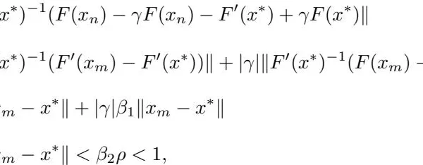
so $x_{1} \in U(x_{0}, t^{*})$ . Suppose (2.13) holds for all values of $m$ smaller or equal to $n - 1$ . Next, we show $A_{m + 1} \neq 0$ . Using the definition of $A_{m + 1}$ , (A2), (A3) we get in turn that

where we also used by the induction hypotheses that

so $x_{m + 1} \in U(x_0, t^*)$ . It also follows from (2.14) that $A_{m + 1} \neq 0$ and

by the Banach lemma on inverses of functions [8]. Moreover, we can write by method (1.2):

since $F(x_{m}) = -(F^{\prime}(x_{m}) - \gamma F(x_{m}))(x_{m + 1} - x_{m})$ . By (A3) and (2.16), we obtain in turn

It then follows from (1.2), (2.15) and (2.17) that

and

But sequence $\{t_m\}$ is fundamental. So, sequence $\{x_{m}\}$ is fundamental too (by (2.18)), so it converges to some $x^{*}\in U[x_{0},t^{*}]$ . By letting $m\longrightarrow \infty$ in (2.17), we deduce that $F(x^{*}) = 0$ .

Next, we present a uniqueness of the solution result for equation (1.1).

Proposition 2.4 Suppose

(1) There exists $x_0 \in D, K > 0$ such that $F'(x_0) \neq 0$ and

for all $v\in D$

(2) The point $x^{*} \in U[x_{0}, a] \subseteq D$ is a simple solution of equation $F(x) = 0$ for some $a > 0$ . (3) There exists $b \geq a$ such that

Set $B = U[x_0, b] \cap D$ . Then, the only solution of equation $F(x) = 0$ in $B$ is $x^*$ .

Proof. Set $M = \int_0^1 F'(z^* + \theta(x^* - z^*)) d$ for some $z \in B$ with $F(z^*) = 0$ . Then, in view of (2.20)

so, $z^{*} = x^{*}$ follows from $M\neq 0$ and $M(z^{*} - x^{*}) = F(z^{*}) - F(x^{*}) = 0 - 0 = 0$

III. LOCAL CONVERGENCE

Let $\beta_0, \beta$ and $\beta_{1}$ be positive parameters. Set

Define function $h:[0,\frac{1}{\beta_2})\longrightarrow \mathbb{R}$ by

Suppose this function has a minimal zero $\rho \in (0, \frac{1}{\beta_2})$ . We shall use conditions

(H). Suppose:

(H1) The point $x^{*} \in D$ is a simple solution of equation (1.1).
(H2) There exists $\beta_0 > 0$ such that

for all $v\in D$ . Set $D_{1} = U(x^{*},\frac{1}{\beta_{0}})\cap D$

(H3) There exist $\beta > 0, \beta_1 > 0$ such that

and

for all $v, w \in D_1$ .

(H4) Function $h(t) - 1$ has a minimal solution $\rho \in (0,1)$ .

and

(H5) $U[x^{*},\rho ]\subset D$

Notice that $A(x^{*}) = F^{\prime}(x^{*})$ . Then, we get the estimates

leading to

So, we get

and $x_{m + 1}\in U(x^{*},\rho)$ . Hence, we conclude by (3.1) that $\lim_{m\longrightarrow \infty}x_m = x^*$ . Therefore, we arrive at the local convergence result for method (1.2).

Theorem 3.1 Under conditions (H) further suppose that $x_0 \in U(x^*, \rho)$ . Then, sequence $\{x_n\}$ generated by method (1.2) is well defined in $U(x_0, \rho)$ , remains in $U(x_0, \rho)$ and converges to $x^*$ .

Next, we present a uniqueness of the solution result for equation (1.2).

Proposition 3.2 Suppose

(1) The point $x^{*}$ is a simple solution of equation $F(x) = 0$ in $U(x^{*},\tau)\subset D$ for some $\tau >0$ . (2) Condition (H2) holds. (3) There exists $\tau^{*} \geq \tau$ such that

Set $B_{1} = U[x_{0},\tau^{*}]\cap D$ . Then, the only solution of equation (1.1) in $B_{1}$ is $x^{*}$

Proof. Set $M_1 = \int_0^1 F'(z^* + \theta(x^* - z^*)) d$ for some $z^* \in B_1$ with $F(z^*) = 0$ . Then, using (H2), we get in turn that

so, $z^{*} = x^{*}$ follows from $M_1 \neq 0$ and $M_1(z^* - x^*) = F(z^*) - F(x^*) = 0 - 0 = 0$ .

IV. NUMERICAL EXAMPLE

We verify convergence criteria using method (1.2) for $\gamma = 0$ , so $\delta = 0$ .

Example 4.1 (Semi-local case) Let us consider a scalar function $F$ defined on the set $D = U[x_0,1 - q]$ for $q \in (0, \frac{1}{2})$ by

Choose $x_0 = 1$ . Then, we obtain the estimates $\eta = \frac{1 - q}{3}$ ,

for all $x \in D$ , so $L_0 = 3 - q$ , $D_0 = U(x_0, \frac{1}{L_0}) \cap D = U(x_0, \frac{1}{L_0})$ ,

for all $x,y\in D$ and so $L = 2(1 + \frac{1}{L_0})$

Next, set $y = x - F'(x)^{-1}F(x), x \in D$ . Then, we have

Define function $\bar{F}$ on the interval $D = [q,2 - q]$ by

Then, we get by this definition that

where $p = \sqrt[3]{\frac{2q}{5}}$ is the critical point of function $\bar{F}$ . Notice that $q < p < 2 - q$ . It follows that this function is decreasing on the interval $(q,p)$ and increasing on the interval $(q,2 - q)$ , since $x^{2} + xq + q^{2} > 0$ and $x^{3} > 0$ . So, we can set

and

But if $x \in D_0 = [1 - \frac{1}{L_0}, 1 + \frac{1}{L_0}]$ , then

where $\varrho = \frac{4 - q}{3 - q}$ and $K < K_{1}$ for all $q\in (0,\frac{1}{2})$ . For $q = 0.45$ , we have

n	1	2	3	4	5
tn	0.1833	0.2712	0.3061	0.3138	0.3142	0.3142
(L0+\|γ\|δ)tn+1	0.4675	0.6916	0.7804	0.8001	0.8011	0.8011

Thus condition (2.2) satisfied.

Example 4.2 Let $F:[-1,1]\longrightarrow \mathbb{R}$ be defined by

Then, we have for $x^{*} = 0, \beta_{0} = e - 1, \beta = e^{\frac{1}{e - 1}}$ and $\beta_{1} = 0$ . So, we have $\rho = 0.3827$ .

References

10 Cites in Article
Ioannis Argyros (1942). Unified Convergence Criteria for Iterative Banach Space Valued Methods with Applications.
Ioannis Argyros (2008). Newton-like Methods.
Ioannis Argyros,Santhosh George (2021). Mathematical Modeling for the Solution of Equations and Systems of Equations with Applications. Volume IV.
Ramandeep Behl,V Kanwar (2014). New Highly Efficient Families of Higher-Order Methods for Simple Roots, Permitting<mml:math xmlns:mml="http://www.w3.org/1998/Math/MathML" id="M1"><mml:mrow><mml:msup><mml:mi>f</mml:mi><mml:mo>′</mml:mo></mml:msup><mml:mo stretchy="false">(</mml:mo><mml:msub><mml:mi>x</mml:mi><mml:mi>n</mml:mi></mml:msub><mml:mo stretchy="false">)</mml:mo><mml:mo>=</mml:mo><mml:mn>0</mml:mn></mml:mrow></mml:math>.
Jisheng Kou,Yitian Li,Xiuhua Wang (2007). A family of fifth-order iterations composed of Newton and third-order methods.
S Kumar,V Kanwar,S Tomar,S Singh (2011). Geometrically constructed families of Newton's method for unconstarined optimization and nonlinear equations.
Muhammad Noor,Khalida Noor (2007). Fifth-order iterative methods for solving nonlinear equations.
J Ortega,W Rheinboldt (2000). Iterative Solution of Nonlinear Equations in Several Variables.
J Traub (1964). Iterative schemes for the solution of equations prentice Hall.
Miodrag Petkovic,Ljiljana Petkovic (2013). Families of optimal multipoint methods for solving nonlinear equations: A survey.
No ethics committee approval was required for this article type.
Data Availability
Not applicable for this article.
How to Cite This Article
Samundra Regmi, Ioannis Argyros, Santhosh George, Christopher Argyros. 2026. "On the Convergence of a Single Step Third Order Method for Solving Equations". Global Journal of Science Frontier Research - F: Mathematics & Decision GJSFR-F Volume 22 (GJSFR Volume 22 Issue F1).
Explore published articles in an immersive Augmented Reality environment. Our platform converts research papers into interactive 3D books, allowing readers to view and interact with content using AR and VR compatible devices.
Your published article is automatically converted into a realistic 3D book. Flip through pages and read research papers in a more engaging and interactive format.