Among electric vehicle charging technologies, wireless charging technology is favored by consumers and car companies for its advantages of simple operation and small space. However, due to low charging efficiency and non-universal charging equipment, wireless charging equipment for electric vehicles has not been effectively promoted. Based on this, integrated circuit theory and electromagnetic field equation, this paper established electromagnetic coupling wireless charging circuit model, based on this model, the maximum wireless charging power transmission efficiency and the maximum horizontal offset and other issues are studied.
## I. RESTATEMENT OF THE PROBLEM
### a) Background
Electric vehicles are favored by consumers because of their advantages over traditional fuel cars. However, the existing wired charging method of ELECTRIC vehicles is complicated in operation and has safety risks. Therefore, the adoption of wireless charging method to charge electric vehicles quickly, safely and conveniently has become the goal pursued by the electric vehicle industry.
Currently, many manufacturers are developing wireless charging technology for electric cars. When the electric car parked in a specific location, power grid through underground launch mechanism of high frequency alternating magnetic field to wireless charging of electric cars, has the advantages of convenient operation, small space occupied, but there are many electric car manufacturers at present, proprietary models must use the special-purpose wireless charging equipment, this causes the waste of electricity. Therefore, it is of great significance to optimize the non-on-board part of wireless charging to make the connectivity between wireless charging equipment and electric vehicles of different manufacturers.
### b) Restatement of the Problem
Wireless charging system is composed of vehicle-mounted part and non-vehicle-mounted part. The on-board part consists of an RLC circuit and a load, and the non-on-board part consists of a power supply and another RLC circuit. Two inductance elements, L_1 (transmitting coil inductance, also known as matching impedance) and L_2 (receiving coil inductance), transmit electrical energy by coupling to produce a magnetic field. It can be assumed that the mutual inductance between the two coils depends only on distance.
A lab conducted 10 experiments to study the transmission efficiency of wireless charging. Known wireless charging vehicle part and ground part at different distances of 10 experimental data. (The experiment was carried out under the condition that the vertical projection of the transmitting and receiving coils overlapped perfectly.) The parameters of the wireless charging ground launcher used in the experiment and the electromagnetic-mechanical adjustable range of the experimental equipment launcher are known.
Problem 1: Under the condition of complete resonance of transmitting and receiving coils, mathematical models of transmitting frequency, matching impedance and radio energy transmission efficiency were established to calculate the power transmission efficiency of 10 experiments of wireless charging.
Problem 2: Due to the design of the electric vehicle itself, the distance between the on-board part of its wireless charging and the ground may be any value within the regulation. The mathematical models of transmitting frequency, matching impedance, distance between two coils and radio energy transmission efficiency are established by modifying the mathematical model of question 1. When the distance between the two coils in the first experiment was changed from $100\mathrm{mm}$ to $150\mathrm{mm}$, $200\mathrm{mm}$ and $250\mathrm{mm}$, the power transmission efficiency of wireless charging was recalculated and compared.
Problem 3: Previous studies have shown that transmission efficiency can be improved by changing transmission frequency and matching impedance. In the first experiment (the distance between the two coils is $100\mathrm{mm}$ ), can transmission efficiency be maximized by adjusting transmission frequency and matching impedance value? What's the maximum?
Problem 4: When the electric vehicle stops for wireless charging, it is difficult to ensure the complete vertical projective overlap between the transmitting coil and the receiving coil, and there will always be more or less deviation. The radius of the coil is $R$, and the center of the receiving coil (h away from the transmitting coil) deviates a (mm) from the positive direction of the X axis. Continuing the research in question 3, please calculate the maximum value of A under the premise that the maximum transmission efficiency is greater than $80\%$ when h is $100\mathrm{mm}$ from the ground vertically.
## II. PROBLEM ANALYSIS
In order to establish the energy transmission model between the transmitting coil and the receiving coil in wireless charging, calculate the power transmission efficiency and optimize the coil design, the four questions given by the topic are analyzed.
### a) Analysis of Problem 1
It is clear that the circuit is in full resonance, that is, the transmitting frequency is the resonant frequency of the RLC oscillation circuit. In order to calculate the power transmission efficiency of several experiments, a linear equation containing coupling coefficient and circuit quality factor should be established based on kirchhoff equation and grid analysis theory. After solving the linear equation, the power transmission efficiency can be obtained by substituting the experimental parameters.
### b) Analysis of Problem 2
Question 2 On the basis of question 1, it is necessary to further explore the influence of distance between two coils on power transmission efficiency. In view of the distance only affects the mutual inductance between the two coils, but does not affect the circuit quality factor, capacitance and inductance value. Therefore, this question only explores the relationship between mutual inductance and distance. In order to get the relationship between the two, it is necessary to derive the relationship between mutual inductance and distance based on electromagnetic theory, then determine the parameters by fitting, and substitute the obtained relationship into the model obtained in question 1 to calculate the electric energy transmission efficiency.
### c) Analysis of Problem 3
In the third problem, it is necessary to adjust the transmission frequency and matching impedance on the basis of the fixed distance between the two coils to maximize the transmission efficiency. Using the model of problem 1, it can be seen that the matching impedance affects the resonant frequency of the circuit, thus affecting the quality factor of the circuit, and the transmission frequency affects the calculation of parameter A, both of which will affect the power transmission efficiency. Considering that the range of transmission frequency and matching impedance given by the problem is not large, the ergodic method can be adopted to find the optimal solution.
### d) Analysis of Problem 4
The fourth problem needs to find the maximum value of horizontal offset under the condition that the maximum transmission efficiency is greater than $80\%$ on the basis of the fixed vertical distance between the two coils. Considering that distance will affect mutual inductance between two coils, horizontal offset will cause mutual inductance change. Referring to the models in question 1 and 3, it can be seen that the transmission frequency, matching impedance and horizontal offset distance need to be adjusted to find the maximum power transmission efficiency. Due to the large number of optimization variables and large search space, simulated annealing algorithm can be used for global optimization to find the maximum horizontal offset distance that meets the requirements.
## III. PROBLEM ANALYSIS
Due to the complexity of the energy coupling transfer process of the actual electromagnetic system and the limited data provided by the topic, the following hypotheses are proposed in order to better understand the physical nature of the problem and simplify the model:
1. The circuit is a lumped parameter circuit, that is, the voltage between any two endpoints of the circuit and the current flowing into any device terminal knob are completely determined, independent of the geometric size and spatial position of the device.
2. Electromagnetic coupling in a circuit occurs only between the transmitting coil and the receiving coil. The energy transfer losses between the power supply and the transmitting coil, the receiving coil and the load, and the two RLC circuits are negligible, and their coupling coefficient is considered to be 1. For mutual inductance between two coils, mutual inductance is only related to the distance between them.
3. For coils, it is considered that the inductance does not change significantly at the frequency set in the topic. The coil is regarded as an ideal hollow solenoid structure without considering the shape and edge effect of the coil. The influence of the distributed capacitance of the coil on the model is not considered.
4. For the receiving coil, the resistance is considered to be $0.2\Omega$ Generally speaking, the resistance of the solenoid wound by copper wire is less than 1. The solenoid turns of the general wireless charging device is 10 turns, and the calculated resistance is about $0.1 \sim 0.2\Omega \Omega$. This paper discusses this problem at the end.
## IV. SIGN EXPLANATION AND NOUN EXPLANATION
Table 1: Symbol description
<table><tr><td>Symbol</td><td>Instructions</td><td>Unit</td></tr><tr><td>L1</td><td>Transmitting inductance</td><td>H</td></tr><tr><td>L2</td><td>Inductance of receiving coil</td><td>H</td></tr><tr><td>Q1</td><td>Transmitting loop RLC circuit quality factor</td><td>1</td></tr><tr><td>M</td><td>Mutual inductance</td><td>H</td></tr><tr><td>j</td><td>Imaginary unit</td><td>There is no</td></tr><tr><td>k12</td><td>The coupling coefficient</td><td>1</td></tr><tr><td>η</td><td>Power transmission efficiency</td><td>1</td></tr><tr><td>t0</td><td>Initial temperature in simulated annealing algorithm</td><td>1</td></tr><tr><td>kt</td><td>Probability coefficient of temperature</td><td>1</td></tr></table>
## V. THE ESTABLISHMENT AND SOLUTION IF THE MODEL
a) Problem 1: two-port network model of wireless charging
i. Model preparation In order to study the electromagnetic energy transmission process between transmitting loop and receiving loop, this paper needs to model the electromagnetic energy distribution of transmitting loop, receiving loop and intermediate transmission process. Before modeling, some basic laws of circuit theory and basic conclusions of common circuits are introduced.
1. Lumped hypothesis: the circuit can be divided into lumped parameter circuit and distributed parameter circuit according to the relationship between the geometrical dimension of the actual circuit and the working signal wavelength. dλ The lumped parameter circuit corresponds to the circuit satisfied, that is, the size of the device is far less than the wavelength corresponding to the normal operating frequency of the circuit. d << λln lumped parameter circuits, the concepts of voltage and current can be used to describe the circuit without the distribution of electric and magnetic fields along the circuit. Generally speaking, the circuit whose operating frequency is less than 20MHz can be called the low-frequency circuit, and the low-frequency circuit applies to lumped hypothesis.
2. Kirchhoff's current law: At any moment in a lumped parameter circuit, assuming that the current entering a node is positive and the current leaving the node is negative, the algebraic sum of all currents involved in the node is equal to zero. That is, the current flowing into the node must equal the current flowing out of the node. Kirchhoff's current law reflects the conservation of current.
3. Kirchhoff's voltage law: in lumped circuit, the algebraic sum of the voltages of each branch is equal to zero at any time, along any closed path. Kirchhoff's voltage law reflects the conservation of energy.
4. Sinusoidal and phasor method: in actual AC, voltage and current often change in sinusoidal way, called as the amount of sinusoidal, which is called the effective value of the sinusoidal, is the circular frequency of the sinusoidal, is the initial phase. $\mathbf{i}(\mathbf{t}) = \sqrt{2}\mathbf{I}\cos (\omega t + \varphi)\mathbf{I}\omega \varphi$ For circuit contains only the linear element of linear circuit (i.e., passive component contains only resistor, inductor and capacitor circuit), the circuit equations can be expressed as the linear ordinary differential equation, the solution for convenient, often think of sine using euler's formula is expressed as the plural, namely the definition, which for the plural unit (avoid confused with current without using), called the phasor. $\dot{\mathbf{l}} = \mathbf{l}\angle \varphi = \mathbf{I}\mathbf{e}^{\mathrm{j}\varphi}\mathbf{j}\mathrm{i}\mathbf{i}\mathbf{l}$ Using the concept of phasor, differential equation can be transformed into algebraic equation, which is easy to solve.
5. Capacitive reactance and inductive reactance: when applying the phasor method to solve the circuit, the inductance and capacitance can be defined as impedance, following the definition of resistance, to facilitate the solution. $\dot{\mathbf{U}} /\dot{\mathbf{I}}$ For the inductance, by definition, it is called the inductive reactance of the inductance, whose dimension is (ohm); $\dot{\mathbf{U}} =$ $\mathrm{j}\omega \mathrm{L}\dot{\mathrm{IX}}_{\mathrm{L}} = \omega \mathrm{L}\Omega$ For capacitance, by definition, it is called the capacitance reactance, which has dimension (ohm). $\dot{\mathbf{U}} = \frac{1}{\mathrm{j}\omega\mathrm{C}}\dot{\mathrm{IX}}_{\mathrm{C}} = -1 / (\omega \mathrm{C})\Omega$
6. Two-port network: the actual circuit is generally complicated. In order to understand the input and output functions of the circuit system more clearly, Brisig, 1921[3]It is pointed out that a two-port
network composed of linear elements can always be described by a set of equations regardless of its internal structure and parameters. The internal structure of the circuit is regarded as a black box,
## ii. Model establishment
and the function of the system is studied through the relationship between different inputs and outputs.
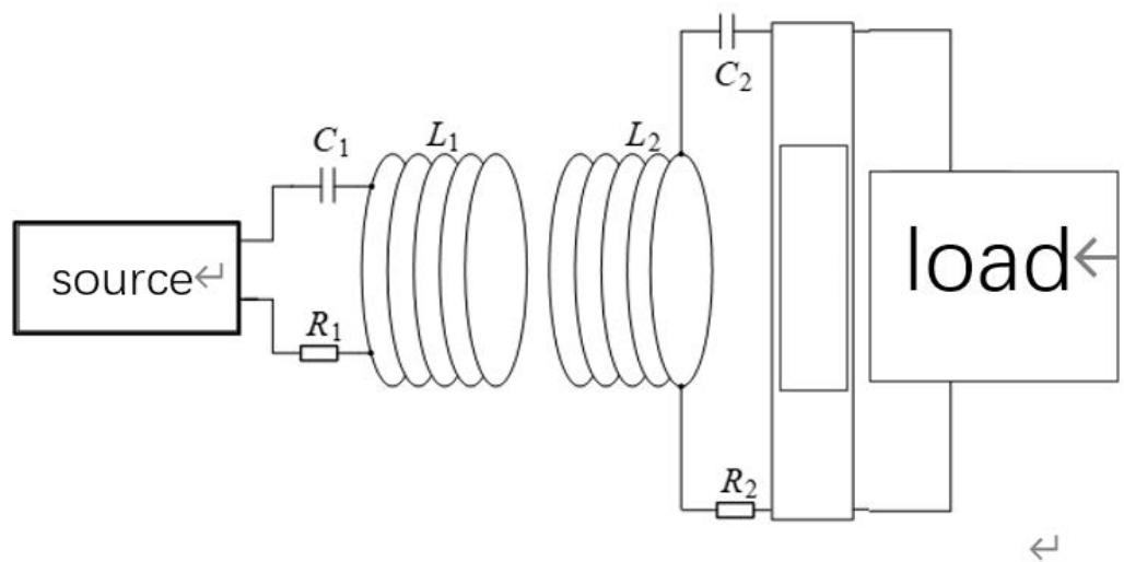
 Fig. 1: Structural equivalent diagram of wireless charging system
As shown in Figure 1, the wireless charging process of ev is simplified into vehicle-mounted part and non-vehicle-mounted part, wherein the vehicle-mounted part is composed of an RLC circuit and load, and the non-vehicle-mounted part is composed of power supply and an RLC circuit.
First, the interaction between two inductors is dealt with. Consider the simplified circuit as shown
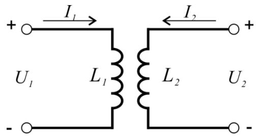 Fig. 2: Interaction circuit between inductors
Using Kirchhoff's voltage law, we know that
$$
U _ {1} = L _ {1} \frac {d i _ {1}}{d t} + M \frac {d i _ {2}}{d t}, U _ {2} = L _ {2} \frac {d i _ {2}}{d t} + M \frac {d i _ {1}}{d t}
$$
Perform the identity transformation, then
$$
U _ {1} = (L _ {1} - M) \frac {d i _ {1}}{d t} + M \frac {d (i _ {1} + i _ {2})}{d t}
$$
$$
U _ {2} = (L _ {2} - M) \frac {d i _ {2}}{d t} + M \frac {d (i _ {1} + i _ {2})}{d t}
$$
Thus, the circuit shown in Figure 2 can be transformed into a T-shaped equivalent circuit, as shown in Figure $3^{[4]}$.
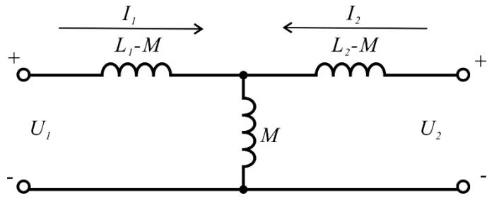 Fig. 3: T-shaped equivalent circuit
In this case, it is necessary to add elements such as resistors and capacitors on the basis of the t-shaped equivalent circuit. For wireless charging of electric vehicles, there are four common capacitive connection modes, namely SS (primary series-secondary series), SP (primary series-secondary parallel connection), PS (primary series-secondary series connection), and PP (primary series-secondary parallel connection).[1]. In this case, the load resistance is large, and only THE SP connection mode has a strong load capacity. Therefore, the SP connection mode is selected, and the equivalent circuit obtained is shown in Figure 4. Where are resistors in RLC circuit respectively, and are circuit load. $R_{1}, R_{2}R_{L}$
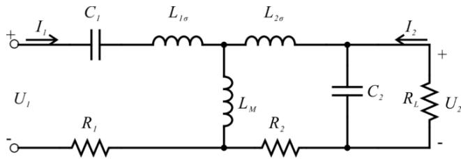 Fig. 4: Two-port network model of wireless charging system
Based on the foregoing results, it can be known that. Define the coupling coefficient, the ratio of turns, the ratio of effective turns. Specify the inflow direction as the current reference direction. $L_{1\sigma} = L_1 - M,L_{2\sigma} = L_2-$ $M,L_{M} = Mk_{12} = \frac{M_{12}}{\sqrt{L_{1}L_{2}}} n = N_{2} / N_{1}n_{e} = L_{2} / L_{1}$ Using Kirchhoff's law, it can be deduced that (equality in a matrix is phasor, the same as below) $V_{1},I_{1}$
$$
\left(V _ {1} = a _ {1 1} V _ {2} + a _ {1 2} (- I _ {2}) \right.
$$
$$
\left\{I _ {1} = a _ {2 1} V _ {2} + a _ {2 2} (- I _ {2}) \right\}
$$
Written in matrix form, then
$$
\left[ \begin{array}{c} V _ {1} \\I _ {1} \end{array} \right] = \left[ \begin{array}{c c} a _ {1 1} & a _ {1 2} \\a _ {2 1} & a _ {2 2} \end{array} \right] \left[ \begin{array}{c} V _ {2} \\- I _ {2} \end{array} \right]
$$
Call the coefficient matrix the A-parameter matrix. For the circuit shown in Figure 4, the calculation can be obtained
$$
\left\{
\begin{array}{c}
a_{11} = \omega^{2} M C_{2} + \frac{1}{M} \left(\frac{C_{2}}{C_{1}} - \omega^{2} L_{1} C_{2} + j \omega R_{1} C_{2}\right) \left(\frac{R_{2}}{j \omega} + L_{2} - \frac{1}{\omega^{2} C_{2}}\right) \\
a_{12} = - j \omega M + \frac{1}{M} \left(L_{1} + \frac{R_{1}}{j \omega} - \frac{1}{\omega^{2} C_{1}}\right) (j \omega L_{2} + R_{2}) \\
a_{21} = \frac{j \omega}{M} \left(L_{2} C_{2} + \frac{R_{2} C_{2}}{j \omega} - \frac{1}{\omega^{2}}\right) \\
a_{22} = \frac{1}{M} \left(L_{2} + \frac{R_{2}}{j \omega}\right)
\end{array}
\right.
$$
The following is the calculation of power transmission efficiency, which is defined as
$$
\eta = \left| \frac {V _ {2} I _ {2}}{V _ {1} I _ {1}} \right| = \left| \frac {V _ {2}}{V _ {1}} \right| \left| \frac {I _ {2}}{I _ {1}} \right|
$$
Define voltage transfer coefficient, current transfer coefficient, then. By using the definition of parameter A, it can be known that $K_{V} = V_{2} / V_{1}|K_{I} = I_{2} / I_{1}|\ \eta = K_{V}K_{I}$
$$
K _ {V} = \left| \frac {V _ {2}}{a _ {1 1} V _ {2} + a _ {1 2} (- I _ {2})} \right| = \left| \frac {1}{a _ {1 1} + a _ {1 2} / R _ {2}} \right|
$$
$$
K _ {I} = \left| \frac {I _ {2}}{a _ {2 1} V _ {2} + a _ {2 2} (- I _ {2})} \right| = \left| \frac {- 1}{a _ {2 2} + a _ {2 1} R _ {2}} \right|
$$
The power transmission efficiency can be obtained by substituting the calculation result of parameter A before.
## iii. Model solution and results
According to problem 1, the circuit is in complete resonance state during the experiment, that is, the transmitting loop and receiving loop are in resonance state at this time, then the capacitance can be calculated. Based on the above discussion, the solution process can be defined as follows: $2\pi f_{0} = \frac{1}{\sqrt{LC}}$
1. Step 1: calculate the coupling coefficient and quality factor according to the experimental data. $k_{12} Q$
2. Step 2: solve A parameter matrix.
3. Step 3: calculate the voltage transmission coefficient and current transmission coefficient, and then calculate the power transmission efficiency. $\eta$
To calculate efficiency, you also need to determine the receiving loop coil resistance. In general, Refs $R_{2}R_{2} \ll R_{L}^{[1]}$ In this paper, the sensitivity analysis is carried out. $R_{2} = 0.2\Omega$ Matlab is used for programming calculation, and the calculation results are shown in Table 2.
Table 2: Calculation results of Problem 1
<table><tr><td>The serial number</td><td>Two coil distance h(mm)</td><td>Transmitting inductance L1 (mu H)</td><td>Inductance of receiving coil L2 (mu H)</td><td>Mutual inductance coil M12 mu (H)</td><td>Transmission efficiency%</td></tr><tr><td>1</td><td>100</td><td>162.21</td><td>163.6</td><td>63.83</td><td>87.90</td></tr><tr><td>2</td><td>125</td><td>161.46</td><td>163.04</td><td>51.49</td><td>86.47</td></tr><tr><td>3</td><td>150</td><td>161.36</td><td>163.15</td><td>40.17</td><td>84.17</td></tr><tr><td>4</td><td>175</td><td>161.75</td><td>162.87</td><td>33.24</td><td>82.73</td></tr><tr><td>5</td><td>200</td><td>161.79</td><td>162.96</td><td>28.24</td><td>80.06</td></tr><tr><td>6</td><td>225</td><td>161.59</td><td>163.15</td><td>26.17</td><td>78.17</td></tr><tr><td>7</td><td>250</td><td>161.53</td><td>163.25</td><td>24.78</td><td>76.82</td></tr><tr><td>8</td><td>275</td><td>161.35</td><td>162.72</td><td>22.12</td><td>74.52</td></tr><tr><td>9</td><td>300</td><td>162.61</td><td>163.74</td><td>21.25</td><td>73.61</td></tr><tr><td>10</td><td>325</td><td>161.39</td><td>163.26</td><td>20.53</td><td>71.93</td></tr></table>
### b) Problem two: model of mutual inductance varying with distance
## i. Model establishment
The change of the distance between the two coils will directly affect the mutual inductance, and then affect the power transmission efficiency through the coupling coefficient. As shown in FIG. 5, the axis is taken as the vertical axis, and the two coils are apart and there is no deviation in the plane. $zhx - y$ The radius of each coil is $P$ and $Q$ are points on each coil. $r = 35mm$ Let the turns of the two coils be respectively and $N_{1}N_{2}$
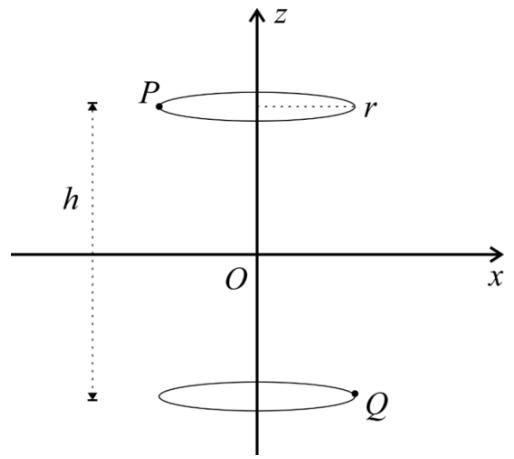 Fig. 5: Geometric diagram of the vertical distance of two coilsh
The cylindrical coordinate system is adopted, the coordinate of point $\mathbb{P}$ is, the coordinate of point $\mathbb{Q}$ is, then the distance between two points satisfies $(r_1, \theta_1, z_1)(r_2, \theta_2, z_2) \mathcal{D}$
$$
\mathcal {D} = [ 2 r ^ {2} - 2 r ^ {2} \cos (\theta_ {2} - \theta_ {1}) + h ^ {2} ] ^ {\frac {1}{2}}
$$
Use the Neumann formula[5], mutual inductance between coaxial circular coils can be expressed as
$$
M = \frac {\mu_ {0} N _ {1} N _ {2}}{4 \pi} \oint_ {l _ {1}} \oint_ {l _ {2}} \frac {d \overrightarrow {l _ {1}} \cdot d \overrightarrow {l _ {2}}}{\mathcal {D}}
$$
Where respectively represent the circumference of the two coils, respectively are the elements on the coils. $l_{1}, l_{2} \vec{d l_{1}}, d \vec{l_{2}}$ Using Figure 5, can be obtained
$$
M = \frac {\mu_ {0} N _ {1} N _ {2}}{4 \pi} \int_ {0} ^ {2 \pi} d \theta_ {2} \int_ {0} ^ {2 \pi} \frac {r ^ {2} \cos (\theta_ {2} - \theta_ {1}) d \theta_ {1}}{\sqrt {2 r ^ {2} - 2 r ^ {2} \cos (\theta_ {2} - \theta_ {1}) + h ^ {2}}}
$$
Plug in the parameters and use the computer to solve the integral. From the integral form, should be inversely proportional to, this conclusion conforms to physical intuition. $Mh$ The resulting curve after plugging in the parameters is shown in the figure. $h - M$
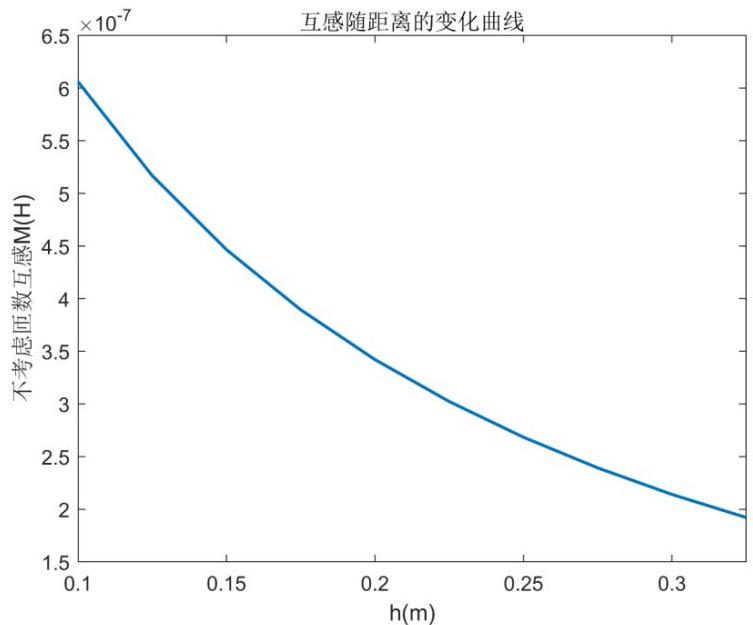 Fig. 6
## ii. Model calculation
The model obtained based on Question 1 and the mutual-inductance model established above varies with distance. In order to calculate the power transmission efficiency when different distances are changed under the first experimental condition, the solving process is formulated as follows:
1. Step1: use integral formula, substitute in known experimental parameters, calculate. $M_{calc}$
2. Step2: Fit and calculate. $M_{calc}M_{Question}N_1N_2$
3. Step3: use the obtained model and substitute it into the model in the first question to set parameters and calculate the electric energy transmission efficiency.
$$
N _ {1} N _ {2} M _ {c a l c}
$$
## iii. The model results
In this paper, the distance provided by the experiment is firstly used to calculate the theoretical mutual inductance value without considering the number of turns. The results are shown in Table 3. $M_{calc}$
Table 3: Theoretical mutual inductance values calculated without considering the number of turns
<table><tr><td>H/mm distance</td><td>100</td><td>125</td><td>150</td><td>175</td><td>200</td><td>225</td><td>250</td><td>275</td><td>300</td></tr><tr><td>Theoretical mutual inductance without considering the number of turns Mcalc/10-7H</td><td>6.060</td><td>5.168</td><td>4.465</td><td>3.894</td><td>3.421</td><td>3.023</td><td>2.684</td><td>2.393</td><td>2.140</td></tr></table>
In order to determine the number of turns, this paper makes a linear fitting between the above obtained values and the measured values. $N_{1}N_{2}M_{calc}$ The result is shown in Figure 6.
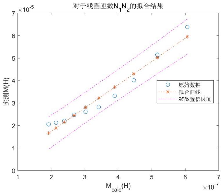 Fig. 6: Fitting results for the number of turns of the coil
$N_{1}N_{2}$
The results show that the expression obtained by fitting is, i.e., given that integer should be taken and 103 is prime, this paper selects the following formula in the subsequent calculation. $y = 103.5x - 3.223 \times 10^{-6}N_{1}N_{2} = 103.5N_{1}N_{2}N_{1}N_{2} = 104$
The relevant information of the fitting is shown in Table 4. It can be seen from the table that the fitting effect is very good. Therefore, the model in this section can be used to describe the relationship between mutual inductance and distance.
Table 4: Fitting evaluation
<table><tr><td>And variance (SSE)</td><td>R2</td><td>Adjusted R2</td><td>Root mean square (RMSE)</td></tr><tr><td>8.283 x 10-11</td><td>0.9562</td><td>0.9508</td><td>3.218 x 10-6</td></tr></table>
Finally, according to the requirements of the question, we calculated the results of the distance of
100mm, 150mm, 200mm and 250mm in the first experiment. See Table 5.
Table 5: Calculation results of question 2
<table><tr><td>H/mm distance</td><td>100</td><td>150</td><td>200</td><td>250</td></tr><tr><td>Transmission efficiency (%)</td><td>87.90</td><td>86.02</td><td>83.35</td><td>79.61</td></tr></table>
### c) Problem three: emission frequency and matching impedance optimization model
## i. Model establishment
Under the condition of constant distance, mutual inductance remains constant. According to the theoretical analysis of problem 1, the change of can directly affect the parameter matrix $A$, and then affect the power transmission efficiency. $L_{1}, f$ Therefore, it is possible to improve transmission efficiency by adjusting transmission frequency and matching impedance.
In view of the complex form of parameter matrix $A$, it is very tedious and unnecessary to work out the relationship between energy transmission efficiency, transmission frequency and matching impedance analytically. Considering that the range of change is not large, we can take the way of traversal and use the computer to search for the most efficient point. $f, L_{1}$
## ii. Model calculation
Based on the mathematical model obtained in question 1 and combined with the experimental data of the first experiment, the solving process is formulated as follows.
1. Step 1: use the A parameter matrix obtained in question 1 to define relevant variables and substitute in parameters.
2. Step 2: Set the search step length and traverse all possible combinations to obtain the energy transmission efficiency matrix. $(f, L_{1})\eta_{all}$
3. Step 3: find the maximum value and find the maximum point accordingly. $\eta_{all}$
## iii. The model results
Matlab was used to search for the maximum efficiency, and the search step of transmitting frequency was set to $10\mathrm{Hz}$, and the search step of matching impedance was set to $0.1\mu \mathrm{F}$. The traversal results are shown in Figure 7. As can be seen from the figure, the maximum power transmission efficiency does exist. Detailed calculation results show that the maximum point corresponds to $\mathsf{F} = 29.73\mathrm{kHz},\mathsf{L}_1 = 147.3\mu \mathsf{F}$, the maximum transmission efficiency is $89.32\%$.
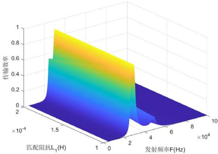 Fig. 7: Results of traversing search for maximum transmission efficiency
Considering that step size setting may affect the traversal search results, this paper sets different search step sizes for emission frequency and matching impedance respectively, and observes the corresponding output results. The calculation results are shown in Table 6.It can be seen from the table that the results obtained under the search step set above are stable, and the search step set above is reasonable.
Table 6: Maximum transmission efficiency obtained at different search steps
<table><tr><td>Transmitting frequency search step (Hz)</td><td>5000</td><td>1000</td><td>100</td><td>50</td><td>10</td><td>1</td></tr><tr><td>Emission frequency search step (μF)</td><td>50</td><td>10</td><td>1</td><td>5</td><td>0.1</td><td>0.01</td></tr><tr><td>Maximum power transmission efficiency (%)</td><td>89.07</td><td>89.07</td><td>89.32</td><td>89.32</td><td>89.32</td><td>89.32</td></tr></table>
### d) Problem four: maximum horizontal migration model
## i. Model establishment
Consider the dislocated coil model shown in Figure 8. The centers of the coils are at $(0,0,0)$ and $(0,a,h)$ respectively. By taking any point $P$ and $Q$ on the two coils and using the rectangular coordinate system, the coordinates of the two points can be expressed as P and Q respectively. $(r\cos \theta_{1},r\sin \theta_{1},0)(r\cos \theta_{2} + a,r\sin \theta_{2},h)$
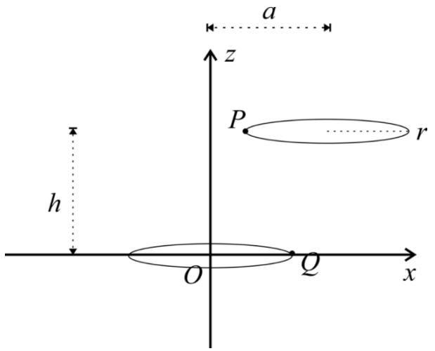 Fig. 8: Misaligned coil model
The distance between two points can be expressed as
$$
\mathcal{D} = \left[ (r \cos \theta_2 + a - r \cos \theta_1)^2 + (r \sin \theta_1 - r \sin \theta_2)^2 + h^2 \right]^{\frac{1}{2}}
$$
By using Neumann formula, mutual inductance between the two coils can be expressed as
$$
M = \frac {\mu_ {0} N _ {1} N _ {2}}{4 \pi} \int_ {0} ^ {2 \pi} d \theta_ {1} \int_ {0} ^ {2 \pi} \frac {r ^ {2} \cos (\theta_ {2} - \theta_ {1}) d \theta_ {2}}{\mathcal {D}}
$$
In terms of integral form, it is inversely proportional to the horizontal offset distance. ML After substituting parameters, the relationship curve between M and horizontal offset obtained is shown in FIG. 9.It can also be seen from the figure that mutual inductance is even function of horizontal offset distance, which is consistent with physical intuition.
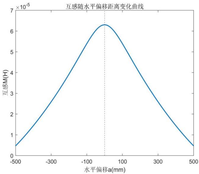 Fig. 9: Variation curve of mutual inductance with horizontal deviation
## ii. Model calculation
Based on the variation of mutual inductance with horizontal migration, a computer can be used to search various combinations of emission frequency, matching impedance and horizontal distance. Considering the large search space, this paper uses simulated annealing algorithm to find the optimal solution.
The idea of the simulated annealing algorithm is derived from the solid annealing process: the solid is heated to a high enough temperature, and then it is cooled slowly. During heating, the particles inside the solid become disordered as the temperature rises, and the internal energy increases. Then, when the particles are cooled slowly, the arrangement gradually tends to be orderly, and finally reaches the ground state at room temperature, and the internal energy decreases to the minimum. Solid annealing process was used to simulate combinatorial optimization problem, the internal energy $E$ simulation as the objective function, the corresponding metal objects combinatorial optimization problem, the corresponding state, optimal solutions corresponding to the lowest energy state, the temperature evolution $T$ for control parameters, according to the boltzmann distribution, the temperature reached its lowest point, obtain the optimal solution of probability is the largest. In simulated annealing algorithm, the introduction of Metropolis acceptance criterion makes the algorithm appear to jump, thus reducing the dependence on the initial solution. The traditional simulated annealing algorithm is:
1. Initial cooling schedule [(initial temperature), (Markov chain length), (temperature attenuation factor), S (stop criterion)], initial solution =; $t = t_0 L_k \alpha x_i x_0$
2. If the number of internal cycles reaches at this temperature, then turn to $3; L_{k}$. Otherwise, determine the chosen neighborhood structure (2_opt or 3_opt), generate a new solution randomly from the neighborhood, calculate $\bar{\delta} f() - f$, if $\bar{\delta}$, then; $x_{j}f_{ij} = x_{j}x_{i}f_{ij} \leq 0$ and $\bar{\delta} f() - f$, otherwise, at that time, make; $\exp(-\Delta f_{ij} / t) > \text{random}(0,1)x_{j} = x_{i}$. Repeat 2;
3. If the stop criterion S is met, the calculation is terminated; Otherwise $= \alpha - 1$, go to 2; $t_k t_k$
4. Output the optimal solution. Intuitively, for each value of the control parameter $T$, the algorithm continues the process of generating new solution-judge-accept/reject.
Based on the traditional simulated annealing algorithm and combined with the actual situation, the solution process is formulated as follows:
1. Step1: Determine the solution space. According to FIG. 9 and the requirements of the problem, considering symmetry, the solution space is defined
as, and the initial solution is set as. $S = \{a|0\leq a\leq$ 10000}x i = 0
1. Step 2: set the objective function. We know that the objective function is $f(x) = x$
2. Step 3: generate a new solution. First, a quantity subject to a normal distribution centered on the average distance is generated to generate a random number of 0-1.dxIf the random number is greater than 0.5, dx is negative; otherwise, dx is positive. Finally, the new solution is $\mathbf{x_j} = \mathbf{x_i} + \mathbf{dx}$
3. Step 4: define constraints. Different from the general simulated annealing case, the new solution needs to be satisfied
$$
\left\{ \begin{array}{l} 0 \leq x_j \leq 10000 \\ \max \eta \geq 80\% \end{array} \right.
$$
If the constraint conditions are met, the new solution is accepted, otherwise a new solution is generated until the condition is met. $x_{j}$
Step 6: solve iteratively until finding the optimal solution that meets the conditions.
## iii. The model results
Using Matlab programming, the maximum value satisfying the problem conditions is 286.0349mm. At this time, mutual inductance is obtained. When the maximum power transmission efficiency is achieved, the transmission frequency is $29.85\mathrm{kHz}$, the matching impedance is $166.6\mu \mathrm{H}$, and the maximum power transmission efficiency is $80.55\%$, which meets the requirements of the problem. $aM = 27.67\mu H$
## VI. SENSITIVITY ANALYSIS
In the above paper, two parameters and are estimated. $N_{1}N_{2}R_{2}$ This section will discuss parameter Settings and conduct sensitivity analysis.
### a) Analysis of parameters $N_{1}N_{2}$
$N_{1}, N_{2}$ Is the number of turns of transmitting coil and receiving coil respectively. In question 2, in order to obtain the model of mutual inductance changing with distance, this paper adopts the fitting method to estimate. $N_{1}N_{2} \approx 103.5$ Considering that they are all integers and 103 is a prime number, the integer is 104. From the fitting effect, it is relatively consistent with the experimental data. $N_{1}, N_{2}N_{1}N_{2} = 104$
In order to quantitatively measure the impact of calculation errors on the results, the power transmission efficiency under the first experimental condition was calculated, assuming a fluctuation of $5\%$, as shown in FIG. 10. $N_{1}N_{2}N_{1}N_{2}N_{1}N_{2} \in [98,110]$
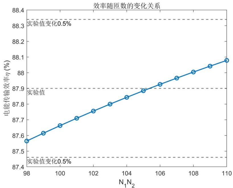 Fig. 10: Sensitivity analysis of the number of turns
As can be seen from the figure, when the number of turns changes by $5\%$, relative to problem 1, the efficiency obtained through measured mutual inductance only changes by less than $0.5\%$. Therefore, the power transmission efficiency is not sensitive to the change of the number of turns, and the model has good stability.
### b) Analysis of parameters $R_{2}$
$R_{2}$ Is the resistance of the coil in the receiving loop. In general, the resistance is less than. Make an estimate. Assume that the coil material is made of copper wire, the cross-sectional area of the wire is, and as discussed above, let the number of turns be 10, then the coil resistance is $110^{-6}\mathrm{m}^2$
$$
R = \frac {2 \pi r \rho N}{S}
$$
Access to information[6]After that, the resistivity of copper is. Therefore, the model is more reasonable. $16.8\mathrm{n}\Omega \cdot \mathrm{m}R\approx 0.13\Omega R_2 = 0.2\Omega$
In order to measure the influence of changes on the model results, a fluctuation of $5\%$ is assumed, i.e., to calculate the electric energy transmission efficiency under the first experiment. The results are shown in FIG. 11. $R_{2}R_{2}R_{2}\in [0.19,0.21]$
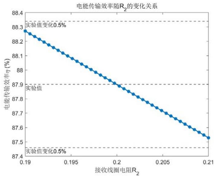 Fig. 11: Sensitivity analysis of pairs
$R_{2}$
Therefore, when the change is $5\%$, the power transmission efficiency changes only $0.5\%$, the power transmission efficiency is not sensitive to the change, and the model has good stability. $R_{2}R_{2}$
## VII. EVALUATION AND EXTENSION OF THE MODEL
### a) Model advantage
In problem 1, this paper constructs a two-port network model of wireless charging. Based on the basic knowledge of circuit theory, the model regarded the complex power transmission system as A black box, constructed parameter A, and then solved according to the specific circuit structure. The modeling idea changed from general to specific, and the obtained solution met the expectation, and the model had good expansibility.
In the second problem, the model of mutual inductance changing with distance is built, the Neumann formula is used to deduce the relationship between mutual inductance and distance, the unknown parameters are determined by fitting, and the computer numerical solution is used, the results are relatively accurate. The accuracy of the fitting process is analyzed, and the sensitivity of the fitting results is analyzed. The model has good stability.
In the third problem, the optimization model of transmission frequency and matching impedance is constructed. The ergodic method is used to search for the optimal combination of transmission frequency and matching impedance under the premise of constant coil distance, and the highest power transmission efficiency is obtained. The modeling method is simple, the calculation speed is fast, and it can be conveniently applied to practical projects.
In problem 4, the maximum horizontal migration model is constructed. The simulated annealing algorithm is used to find the optimal solution for the problem that there are many optimization variables and large search space. The simulated annealing algorithm can jump out of the local optimal solution and obtain the global optimal solution. Moreover, the algorithm has strong robustness and can resist the influence of external unstable factors on the results. The final solution conforms to the physical intuition and meets the requirements of the problem.
### b) Lack of model
In question 2, Neumann formula was used to calculate the multi-turn solenoid and simplify it into a single coil. The size and shape of the multi-turn coil were not considered, and the edge effect was not taken into account. Therefore, the results obtained had certain deviation from the reality.
In question 4, when the simulated annealing algorithm is used for calculation, because the simulated annealing algorithm is affected by the temperature cooling rate, the cooling rate is slow, the search time is long, and the better solution can be obtained, but the solution time is also long. If the cooling rate is increased, the optimal solution may be skipped. Therefore, in practice, in order to obtain the optimal solution, it often takes a long time to calculate.
### c) Model to improve
In view of the shortcomings of the model, this paper puts forward the following improvement directions:
1. In view of the assumption that the coil in the model is an ideal hollow solenoid and the coil shape is not considered and the edge effect is ignored, the mutual inductance between the two actual coils can be calculated using the finite element method subsequently. The finite element calculation results are compared with the results in this paper to explore the reasons for the difference and the impact of the edge effect on power transmission.
2. In view of the assumption that the coupling coefficient between each circuit link in the model is 1, if the coupling coefficient does not meet the requirement of 1, the actual coupling coefficient can be obtained by searching the parameter manual for simple circuit equivalence. For example, the transmitting circuit and the power supply can be treated as series or parallel, and the same is true for the receiving coil and the load. In this way, the efficiency calculation results are more accurate.
3. In view of the problem that the mutual inductance in the model is only related to distance and may fail in the presence of magnetic media (such as iron core), when the relative position of the coil is fixed, the corresponding mutual inductance value can be measured by sensor, and the transmission efficiency can be calculated by using the calculation formula in this paper. If there is relative movement between coils, the relationship between mutual inductance and distance and Angle can be measured by numerical simulation or sensor measurement, and then the transmission efficiency can be calculated by using the formula in this paper.
### d) Model to promote
The mathematical model based on electric vehicle wireless charging two-port network presented in this paper can be applied to other electromagnetic coupling or electromagnetic induction wireless power transmission technologies, and can also be modified to deal with microwave radiation power transmission at high frequencies.
Generating HTML Viewer...
References
6 Cites in Article
Zhu Yong (2016). Research on Wireless Charging System Modeling and Electromagnetic Safety of Electric Vehicle.
He Zhi-Yong (2019). Influence and Optimization of Magnetic Coupling Resonant Radio Energy Transmission Efficiency Based on SS Model.
Wu Xilong (2004). Circuit Analysis.
Zhang Xian (2012). Research on Radio Energy Transmission and Conversion Method based on Electromagnetic mechanical Synchronous Resonance.
Ni Guangzheng (2009). Principle of Engineering Electromagnetic Field.
Connor Electrical Conductivity by Copper --Electrical Conductivity.
No ethics committee approval was required for this article type.
Data Availability
Not applicable for this article.
How to Cite This Article
Fei Shao. 2026. \u201cOptimization and Matching of Electric Vehicle Wireless Charging based on Two-Port Network\u201d. Global Journal of Science Frontier Research - A: Physics & Space Science GJSFR-A Volume 22 (GJSFR Volume 22 Issue A4): .
Explore published articles in an immersive Augmented Reality environment. Our platform converts research papers into interactive 3D books, allowing readers to view and interact with content using AR and VR compatible devices.
Your published article is automatically converted into a realistic 3D book. Flip through pages and read research papers in a more engaging and interactive format.
Among electric vehicle charging technologies, wireless charging technology is favored by consumers and car companies for its advantages of simple operation and small space. However, due to low charging efficiency and non-universal charging equipment, wireless charging equipment for electric vehicles has not been effectively promoted. Based on this, integrated circuit theory and electromagnetic field equation, this paper established electromagnetic coupling wireless charging circuit model, based on this model, the maximum wireless charging power transmission efficiency and the maximum horizontal offset and other issues are studied.
Our website is actively being updated, and changes may occur frequently. Please clear your browser cache if needed. For feedback or error reporting, please email [email protected]
Thank you for connecting with us. We will respond to you shortly.