## I. INTRODUCTION Faults are ubiquitous in complex systems. This article designs efficient fault prevention and repair (FPR) sequencers to prevent faults from occurring and minimize their damage. An FPR sequencer determines the sequence of fault repairs. The cost of faults includes repair costs and damage caused by faults. The repair cost may be assumed to be the same regardless of the sequence of repairs. The damage caused by a fault depends on the time for which the fault exists, which is affected by the FPR sequencer. A fault causes less damage if it is repaired early. A complex system has multiple faults, and there may be a crippling or cascading effect when a few faults occur. Efficient FPR sequencers help reduce damage caused by faults and prevent catastrophic events from occurring. The rest of this article is organized as follows: Section 2 describes related work; Section 3 is the problem statement and formulates the multi-objective FPR model; Section 4 illustrates the methods of FPR; Section 5 presents simulation experiments to validate and identify efficient FPR sequencers; Section 6 discusses important findings; Section 7 illustrates future research directions; and Section 8 concludes the paper. ## II. RELATED WORK Research on efficient fault repair and infrastructure recovery mainly focused on smart grids and highway systems. For example, power-flow models were developed (Ang, 2006; Salmeron et al., 2004) to identify optimal or near-optimal repair sequences for electrical power grids. Fault repair is part of fault management, which uses automated fault detection and diagnostics (Chen and Nof, 2012, 2014, 2015; Nof and Chen, 2015, 2017). An example of fault management is the emergence of the smart grid, which is an electricity network that utilizes digital technology and has the self-detection and self-diagnostics ability. Many organizations (e.g., Electric Power Research Institute (EPRI)) have invested in grid operations and planning to help improve real-time situation awareness, wide area protection and control performance, and the capability to handle extreme events and restore the system (EPRI, 2012). It is a challenging task to prevent and repair faults with an optimal sequence (Ang, 2006; Jin et al., 2018). The FPR problem is prevalent in many systems. Hospitals are entangled in insurance claim denials due to faults in the claim process. Insurance companies are concerned about faults in claims. For instance, FICO (FICO, 2012) developed the Insurance Fraud Manager to detect fraud, abuse, and error in healthcare claims before payment. The result is an unreasonably long delay for many justified payments. Faults in many systems are not efficiently corrected after they are detected. A system may be described with mathematical models. For example, the "scale-free network" depicts electrical power grids (Barabasi and Albert, 1999) and the "random network" depicts transportation networks (Barabasi, 2002; Chen, 2009; Jeong, 2003). These mathematical models may be adapted to depict fault networks. Most methods developed earlier exclusively deal with the repair of a single fault (e.g., Dimitrov et al., 2004; Sim and Endrenyi, 1993). Limited research (Ang, 2006; Salmeron et al., 2004) focused on optimal repair sequences. Previous research (Alizadeh and Sriramula, 2017; Chen, 2009; Chen and Nof, 2012; Nageswara Rao and Viswanadham, 1987; Sanislav et al., 2018) suggested tools to effectively detect, diagnose, and predict multiple faults (conflicts and errors). Several studies (e.g., Dong et al., 2019; Zou et al., 2021) proposed to reconstruct faults for fault diagnostics. This article aims at modeling the fault network and designing the FPR sequencers to prevent faults and minimize the total damage. The methodology applied in this research is part of the effort to control network operations through structural search (Dawande et al., 2011). Structural search is a process to search for useful subsets of nodes in a network. For example, to promote healthy behaviors in social networks (Parsa and Chen, 2013), a subset of a population, i.e., an influential set of opinion leaders and innovators, needs to be identified to maximize the speed and scale of promotion. The primary goal in structural search is to identify useful structures in networks. Moreover, the sequence of operations is of great importance. For example, which node in a terrorist network is removed first and which one is removed next have significant impact on preventing terrorist activities. In an FPR sequencer, the useful structure, i.e., a fault network, is known and comprises all faulty sources and other affected faulty nodes. The sequence of repair, however, needs to be determined. Efficient FPR sequencers designed in this research help advance our understanding of optimizing operations sequences for a useful structure. ## III. PROBLEM STATEMENT ### a) Modeling Fault Networks Nodes in a complex system represent components of the system. Links between nodes represent the flow of products, services, or information. Directed links are arcs. Undirected links are edges (Chen and Nof, 2007, 2010, 2012). If a node $j$ is linked to a node $j'$ directly, there is an arc or an edge between the two nodes. When two nodes $j$ and $j'$ are linked indirectly, there is at least one path between $j$ and $j'$ through other nodesso that products, services, or information can be transmitted from $j$ to $j'$ and/or from $j'$ to $j$. A path does not exist between two nodes if they are not linked directly or indirectly. A fault network is a network of faulty nodes in a system. An edge between two nodes $j$ and $j'$ indicates that a fault at $j$ causes a fault at $j'$ and vice versa; an arc from $j$ to $j'$ indicates that a fault at $j$ causes a fault at $j'$. Figure 1(a) illustrates a system network with 11 nodes. Arcs in the network represent flows of product, service, or information. Figure 1(b) illustrates a fault network of seven faulty nodes in the system described in Figure 1(a). 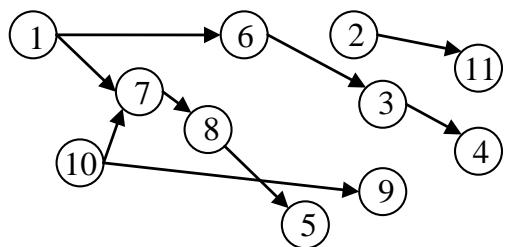 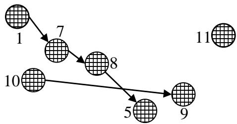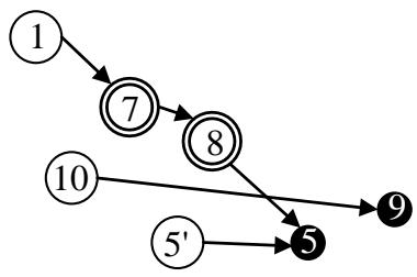(a) A system network  (b) A fault network in the system    Panel label: Root node.  Panel label: Internal node.  Panel label: Leaf node.  (c) A fault network with three types of faulty nodes Figure 1: A system and its network of faulty nodes Root and leaf node The number of arcs connected to a faulty node is the degree of the node (Angeles Serrano and De Los Rios, 2007; Dorogovtsev et al., 2001). The IN degree, $\delta^{IN}$, of a faulty node is the number of arcs that point at the node. The OUT degree, $\delta^{OUT}$, is the number of arcs that originate from the node. There are three types of faulty nodes in a network: leaf, internal, and root nodes. A faulty node $j$ is (a) a root node if its fault is not caused by fault(s) at any other faulty node, $\delta_{j}^{IN} = 0$; (b) a leaf node if it does not cause fault(s) at any other faulty node, $\delta_{j}^{OUT} = 0$; and (c) an internal node when $\delta_{j}^{IN} > 0$ and $\delta_{j}^{OUT} > 0$. A faulty node $j$ is both a root and a leaf node if $\delta_{j}^{IN} = \delta_{j}^{OUT} = 0$; the node is an orphan node because it is not connected to any other nodes. A root node requires repair; an internal or a leaf node is repaired or prevented (from having a failure) if and only if all its causes are repaired or prevented. Nodes 1, 10, and 11 in Figure 1(b), are root nodes and require repair; nodes 7 and 8 are internal nodes; and nodes 5, 9, and 11 are leaf nodes. The total cost of FPR includes repair costs and damage caused by faulty nodes. Repair costs are incurred for all root nodes. All faulty nodes could cause damage, which is reflected on leaf nodes. Suppose node 5 in Figure 1(b) is caused by the faulty node 8 and is also due to a fault that occurs locally at node 5. Figure 1(b) does not show that node 5 requires repair. Repairing node 8 does not remove the fault from node 5. Figure 1(c) clarifies repair requirements by incorporating a pseudo node $5'$ for node 5. Node $5'$ is a root node and requires repair. There are four root nodes (1, 10, 11, and $5'$ ), two internal nodes (7 and 8), and three leaf nodes (5, 9, and 11) in Figure 1(c). Node 11 is both a root and a leaf node. Let $G(W, \mathsf{L})$ represent a complex system where $W$ is a set of nodes (vertices) and $\mathsf{L}$ is a set of links in the system. $|W|$ is the total number of nodes in $W$. $|W|$ is an integer and $|W| > 0$. Since faulty nodes are usually linked through arcs, let $G(V, A)$ represent a directed network of faulty nodes in the system where $V$ is a set of faulty nodes and $A$ is a set of arcs. $|V|$ is the total number of faulty nodes in $V$. $|V|$ is an integer and $|V| \geq 0$. $V \in W$, $A \in \mathsf{L}$, and $|V| \leq |W|$. Let $G(V^F, A^F)$ represent a directed fault network including pseudo nodes. $|V^F| \geq |V|$, $V^F \cap W = V$, and $A^F \cap \mathsf{L} = A$. $|V^F|$ is an integer, and $|V^F| \geq 0$. There are three types of nodes $v_j'$ 's, $v_j \in V^F$: root nodes $v_r'$ 's, internal nodes $v_i'$ 's, and leaf nodes $v_l'$ 's. Let $R, I,$ and $L$ represent a set of root nodes $v_r'$ 's, internal nodes $v_i'$ 's, and leaf nodes $v_l'$ 's, respectively. $|R|, |I|,$ and $|L|$ are integers. $|R| \geq 0$; $|I| \geq 0$; and $|L| \geq 0$. Any FPR sequence must repair all root nodes $v_r'$ 's, $v_i'$ 's and $v_l'$ 's are repaired or prevented if and only if $v_r'$ 's and $v_l'$ 's may be prevented. Time zero, i.e., $t = 0$, is defined to help evaluate the FPR sequences. In practice, the time at which the first fault occurs is often defined as $t = 0$. Let $t_c$ represent the current time and $t_j$ represent the time $v_j$ becomes faulty; $t_c, t_j \geq 0$. Suppose $t_{10} < t_c < t_{9}$ in Figure 1(c). Since $v_9$ has not become faulty at $t_c$, $v_9$ is prevented if $v_{10}$ is repaired before $t_9$. A fault at a root node cannot be prevented because it has already occurred. For any two nodes $v_j$ and $v_{j'}$; $j \neq j'$, $(v_j, v_{j'}) \in A^F$ if $v_j$ directly causes $v_{j'}$. This also implies that $t_j \leq t_{j'}$. COROLLARY 1: In a directed network $G(V^{F}, A^{F})$ of faulty nodes, $t_{j} \leq t_{j'}$ if $(v_{j}, v_{j'}) \in A^{F}$. All $v_{i}$ 's and $v_{l}$ 's, $v_{i} \in I$ and $v_{l} \in L$, are repaired or prevented if and only if all $v_r\text{'s},\v_r\in R,\ \text{are}\ \text{repaired}.\R\cup I\cup L=V^F.\ |R|\leq|V^F|,\ |I|\leq|V^F|,\ \text{and}\ |L|\leq|V^F|.$ There are many network structures. A random network (Erdos and Renyi, 1959; Solomonoff and Rapoport, 1951) follows a degree distribution $\binom{n-1}{d}p^d(1-p)^{n-1-d}$, where $n$ is the total number of nodes, $d$ is the degree of a node or the number of links (arcs or edges) connected to the node, and $p$ is the probability that a pair of nodes are connected. The maximum number of links in a random network is $\frac{1}{2}n(n-1)$. The mean degree $\overline{d}=(n-1)p$. The random network is homogeneous and suitable for modeling networks with approximately the same number of links for each node. The random network has other properties, e.g., a phase transition or bond percolation (Angeles Serrano and De Los Rios, 2007; Newman et al., 2006). These properties are explored in applying FPR sequencers to prevent and repair faults. A scale-free network follows a power law degree distribution $d^{-\gamma}$, where $\gamma$ is between 2.1 and 4. Systems with the structure of a scale-free network are resilient to random faults (Cohen et al., 2000) but are vulnerable to targeted attacks (Cohen et al., 2001). The network structure and its properties underlying a fault network affect the outcome of FPR sequencers and are an integral part of FPR. ### b) Formulating the FPR Model The FPR model has two objectives: (a) minimize total damage, $D$ ( $D \geq 0$ ), caused by faults; and (b) prevent the maximum number of faults from occurring, preventability $P$ ( $0 \leq P \leq 1$ ). The first objective quantifies economic consequences of faults, and the second objective reflects social impacts of faults. Damage is a financial measure whereas preventing faults improves service quality. Let $c_{j}$ represent the time $v_{j}$ is repaired or prevented. $c_{j} < t_{j}$ indicates $v_{j}$ is prevented; $c_{j} > t_{j}$ indicates $v_{j}$ is repaired. Let $p_{j}$ indicate whether $v_{j}$ is prevented. $p_{j} = 0$ if $c_{j} > t_{j}$; $p_{j} = 1$ if $c_{j} < t_{j}$. Since time is continuous, $c_{j} \neq t_{j}$. Preventability $P$ is the percentage of faults that are prevented. $P = \frac{\sum_{j=1}^{|V^F|} p_j}{|V^F|}$. $p_j$ may be expressed in a closed form: $p_j = \frac{c_j - t_j - \sqrt{(c_j - t_j)^2}}{2(c_j - t_j)}$. Let $d_l$ represent the damage caused by $v_l$ over one time unit; $d_l \geq 0$. The damage caused by $v_l$ is $d_l (c_l - t_l)(1 - p_l)$ assuming that $d_l$ is the same over a short period of time $c_l - t l$. The total damage $D = \sum_{l} d_l (c_l - t_l)(1 - p_l)$, $\delta_l^{OUT} = 0$. The objectives of FPR are to minimize $D$ and maximize $P$. The FPR problem is described as a multi-objective optimization model (Eq. (1)): $$ \min \sum_ {l} d _ {l} \frac{c _ {l} - t _ {l} + \sqrt{(c _ {l} - t _ {l}) ^ {2}}}{2} \quad (\text{minimizethetotaldamageD}) $$ $$ \max \sum_ {j = 1} ^ {\left| V ^ {F} \right|} \frac{c _ {j} - t _ {j} - \sqrt{\left(c _ {j} - t _ {j}\right) ^ {2}}}{2 \left| V ^ {F} \right| \left(c _ {j} - t _ {j}\right)} \quad (\text{maximizethepreventability} P) $$ $$ \mathrm{s.t.}c_{j} = \max\left(c_{j^{'}}\right) $$ $$ j = 1, \dots , | V ^ {F} |; (v _ {j ^ {\prime}}, v _ {j}) \in A ^ {F}; \delta_ {l} ^ {O U T} = 0; | V ^ {F} | > 0; d _ {l} \geq 0 \tag {1} $$ $c_{j} = \max \left(c_{j^{\prime}}\right)$ indicates that the time at which $v_{j}$ ( $v_{i}$ or $v_{l}$ ) is repaired or prevented depends on when all its direct causes $v_{j^{\prime}}$ 's are repaired or prevented. For $v_{r}$ 's, $c_{r}$ 's are determined by the FPR sequencer. The decision variables in Eq. (1) are $c_{r}$ 's for $v_{r}$ 's, which are times at which root nodes are repaired. $c_{i}$ 's for $v_{i}$ 's and $c_{l}$ 's for $v_{l}$ 's are determined by $c_{r}$ 's. $d_{l}$ 's, $|V^{F}|$, and $t_{j}$ 's including $t_{l}$ 's are parameters. A feasible solution to Eq. (1) is an FPR sequence that repairs all $v_{r}$ 's. The goal is to identify efficient points, each of which achieves objective function values $D$ and $P$ that are together superior to what can be achieved by all other feasible solutions. Whether an FPR sequence is an efficient point depends on the parameters and topology of fault networks. Both objective functions in Eq. (1) are nonlinear and not differentiable, and the constraints are nonlinear. The model in Eq. (2) rewrites Eq. (1) and admits only linear constraints; the first two objective functions remain nonlinear and not differentiable. Heuristic FPR sequencers and simulation experiments need to be developed to identify and validate efficient sequences. $$ \min \sum_ {l} d _ {l} \frac{c _ {l} - t _ {l} + \sqrt{(c _ {l} - t _ {l}) ^ {2}}}{2} \quad (\text{minimizethetotaldamageD}) $$ $$ \max \sum_ {j = 1} ^ {| V ^ {F} |} \frac{c _ {j} - t _ {j} - \sqrt{\left(c _ {j} - t _ {j}\right) ^ {2}}}{2 | V ^ {F} | \left(c _ {j} - t _ {j}\right)} \quad (\text{maximizethepreventability} P) $$ $$ \min c _ {j} \quad (\text{repaircompletiontimeof} v _ {j}) $$ $$ \mathrm{s.t.}c_{j}\geq c_{j^{ ext{'}}} $$ $$ j = 1, \dots , | V ^ {F} |; (v _ {j}, v _ {j}) \in A ^ {F}; \delta_ {l} ^ {O U T} = 0; | V ^ {F} | > 0; d _ {l} \geq 0 \tag {2} $$ ## IV. METHODS Efficient FPR sequencers prevent faults from occurring and minimize their damage. In many applications, fault repairs are more complex and less automated compared to detection and diagnostics. There are limited resources for FPR. As the order of a fault network increases, more resources are needed to repair faults. With unlimited resources, e.g., unlimited service personnel, all root nodes are repaired simultaneously, which minimizes $D$ and maximizes $P$. When resources are limited, there is a need to design efficient FPR sequencers that minimize $D$ and maximize $P$. Figure 2 shows a fault network of $|R| = 4$ root nodes $v_{1}, v_{2}, v_{3}$, and $v_{4}$, and $|L| = 4$ leaf nodes $v_{5}, v_{6}, v_{7}$, and $v_{8}$, $d_{5}, d_{6}, d_{7}$, and $d_{8}$ are damage per unit time for $v_{5}, v_{6}, v_{7}$, and $v_{8}$, respectively. There are no internal nodes in Figure 2. Let $m_{r}$ represent the time it takes to repair a root node $v_r$; $m_r \geq 0$. $m_1$, $m_2$, $m_3$, and $m_4$ are repair times for $v_1$, $v_2$, $v_3$, and $v_4$, respectively. There are $P_{4,4} = 4! = 24$ possible FPR sequences. In general, there are $|R|$ -permutations of $|R|$ FPR sequences, i.e., $|R|!$ FPR sequences, for a fault network of order $|V^F|$; $|R| \leq |V^F|$. Let $t_0$ represent the time at which an FPR sequence begins repair root node $v_r$; $m_r \geq 0$. $m_1$, $m_2$, $m_3$, and $m_4$ are repair times for $v_1$, $v_2$, $v_3$, and $v_4$, respectively. There are $P_{4,4} = 4! = 24$ possible FPR sequences. In general, there are $|R|$-permutations of $|R|$ FPR sequences, i.e., $|R|!$ FPR sequences, for a fault network of order $|V^F|$; $|R| \leq |V^F|$. Let $t_0$ represent the time at which an FPR sequence begins repairing faults. All 24 FPR sequences and their respective and are summarized in Table 1. 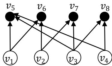 Figure 2: An example of a fault network Table 1: FPR Sequences, Total Damage, and Preventability for the Fault Network in Figure 2 <table><tr><td></td><td>FPR Sequence</td><td>Total Damage D</td><td>Preventability P</td></tr><tr><td>1</td><td>v1→v2→v3→v4</td><td rowspan="4">d5max(m1,2,3,4+t0-t5,0)+d6max(m1,2+t0-t6,0)+d7max(m1,2,3+t0-t7,0)+d8max(m1,2,3,4+t0-t8,0)</td><td>2-|m1,2,3,4+t0-t5|/2(m1,2,3,4+t0-t5)-</td></tr><tr><td rowspan="3">2</td><td rowspan="3">v2→v1→v3→v4</td><td>|m1,2+t0-t6|/2(m1,2+t0-t6)-</td></tr><tr><td>|m1,2,3+t0-t7|/2(m1,2,3+t0-t7)-</td></tr><tr><td>|m1,2,3,t0-t8|/2(m1,2,3,t0-t8)</td></tr><tr><td>3</td><td>v1→v3→v2→v4</td><td rowspan="4">d5max(m1,2,3,4+t0-t5,0)+d6max(m1,2,3+t0-t6,0)+d7max(m1,2,3+t0-t7,0)+d8max(m1,2,3,4+t0-t8,0)</td><td>2-|m1,2,3,4+t0-t5|/2(m1,2,3,4+t0-t5)-</td></tr><tr><td rowspan="3">4</td><td rowspan="3">v3→v1→v2→v4</td><td>|m1,2,3+t0-t6|/2(m1,2,3+t0-t6)-</td></tr><tr><td>|m1,2,3+t0-t7|/2(m1,2,3+t0-t7)-</td></tr><tr><td>|m1,2,3,t0-t8|/2(m1,2,3,t0-t8)</td></tr><tr><td>5</td><td>v1→v2→v4→v3</td><td rowspan="2">d5max(m1,2,3,4+t0-t5,0)+d6max(m1,2+t0-t6,0)+d7max(m1,2,3,4+t0-t7,0)+d8max(m1,2,3,4+t0-t8,0)</td><td rowspan="2">2-|m1,2,3,4+t0-t5|/2(m1,2,3,4+t0-t5)-</td></tr><tr><td>6</td><td>v2→v1→v4→v3</td></tr><tr><td rowspan="5"></td><td rowspan="5"></td><td rowspan="5"></td><td>m1,2+t0-t6/2(m1,2+t0-t6)-</td></tr><tr><td>m1,2,t4+t0-t7/2(m1,2,t4+t0-t7)-</td></tr><tr><td>m1,2,t3,t4+t0-t7/2(m1,2,t3,t4+t0-t7)-</td></tr><tr><td>m1,2,t4+t0-t8/2(m1,2,t4+t0-t8)-</td></tr><tr><td>m1,2,t3,t4+t0-t8/2(m1,2,t3,t4+t0-t8)</td></tr><tr><td>7</td><td>v1→v3→v4→v2</td><td rowspan="5">d5max(m1,2,3,4+t0-t5,0)+d6max(m1,2,3,4+t0-t6,0)+d7max(m1,2,3,4+t0-t7,0)+d8max(m1,3,4+t0-t8,0)</td><td rowspan="2">2-m1,2,3,4+t0-t5/2(m1,2,3,4+t0-t5)-</td></tr><tr><td>8</td><td>v1→v4→v3→v2</td></tr><tr><td>9</td><td>v3→v1→v4→v2</td><td>m1,2,3,4+t0-t6/2(m1,2,3,4+t0-t6)-</td></tr><tr><td rowspan="2">10</td><td rowspan="2">v4→v1→v3→v2</td><td>m1,2,3,4+t0-t7/2(m1,2,3,4+t0-t7)-</td></tr><tr><td>m1,3,4+t0-t8/2(m1,3,4+t0-t8)</td></tr><tr><td>11</td><td>v1→v4→v2→v3</td><td rowspan="4">d5max(m1,2,3,4+t0-t5,0)+d6max(m1,2,4+t0-t6,0)+d7max(m1,2,3,4+t0-t7,0)+d8max(m1,2,3,4+t0-t8,0)</td><td>2-m1,2,3,4+t0-t5/2(m1,2,3,4+t0-t5)-</td></tr><tr><td>12</td><td>v2→v4→v1→v3</td><td>m1,2,4+t0-t6/2(m1,2,4+t0-t6)-</td></tr><tr><td>13</td><td>v4→v1→v2→v3</td><td>m1,2,3,4+t0-t7/2(m1,2,3,4+t0-t7)-</td></tr><tr><td>14</td><td>v4→v2→v1→v3</td><td>m1,2,3,4+t0-t8/2(m1,2,3,4+t0-t8)</td></tr><tr><td>15</td><td>v2→v3→v1→v4</td><td rowspan="4">d5max(m1,2,3,4+t0-t5,0)+d6max(m1,2,3+t0-t6,0)+d7max(m2,3+t0-t7,0)+d8max(m1,2,3,4+t0-t8,0)</td><td>2-m1,2,3,4+t0-t5/2(m1,2,3,4+t0-t5)-</td></tr><tr><td rowspan="3">16</td><td rowspan="3">v3→v2→v1→v4</td><td>m1,2,3+t0-t6/2(m1,2,3+t0-t6)-</td></tr><tr><td>m2,3+t0-t7/2(m2,3+t0-t7)-</td></tr><tr><td>m1,2,3,4+t0-t8/2(m1,2,3,4+t0-t8)</td></tr><tr><td>17</td><td>v2→v3→v4→v1</td><td rowspan="4">d5max(m1,2,3,4+t0-t5,0)+d6max(m1,2,3,4+t0-t6,0)+d7max(m2,3+t0-t7,0)+d8max(m2,3,4+t0-t8,0)</td><td>2-m1,2,3,4+t0-t5/2(m1,2,3,4+t0-t5)-</td></tr><tr><td rowspan="3">18</td><td rowspan="3">v3→v2→v4→v1</td><td>m1,2,3,4+t0-t6/2(m1,2,3,4+t0-t6)-</td></tr><tr><td>m2,3+t0-t7/2(m2,3+t0-t7)-</td></tr><tr><td>m1,2,3,4+t0-t8/2(m2,3,4+t0-t8)</td></tr><tr><td>19</td><td>v2→v4→v3→v1</td><td rowspan="4">d5max(m1,2,3,4+t0-t5,0)+d6max(m1,2,3,4+t0-t6,0)+d7max(m2,3,t0-t7,0)+d8max(m2,3,4+t0-t8,0)</td><td>2-m1,2,3,4+t0-t5/2(m1,2,3,4+t0-t5)-</td></tr><tr><td rowspan="3">20</td><td rowspan="3">v4→v2→v3→v1</td><td>m1,2,3,4+t0-t6/2(m1,2,3,4+t0-t6)-</td></tr><tr><td>m2,3,t0-t7/2(m2,3,t0-t7)-</td></tr><tr><td>m1,2,3,4+t0-t8/2(m2,3,4+t0-t8,0)</td></tr><tr><td>21</td><td>v3→v4→v1→v2</td><td rowspan="4">d5max(m1,2,3,4+t0-t5,0)+d6max(m1,2,3,4+t0-t6,0)+d7max(m1,2,3,4+t0-t7,0)+d8max(m3,4+t0-t8,0)</td><td>2-|m1,2,3,4+t0-t5|/2(m1,2,3,4+t0-t5)-</td></tr><tr><td rowspan="3">22</td><td rowspan="3">v4→v3→v1→v2</td><td>|m1,2,3,4+t0-t6|/2(m1,2,3,4+t0-t6)-</td></tr><tr><td>|m1,2,3,4+t0-t7|/2(m1,2,3,4+t0-t7)-</td></tr><tr><td>|m3,4+t0-t8|/2(m3,4+t0-t8)</td></tr><tr><td>23</td><td>v3→v4→v2→v1</td><td rowspan="4">d5max(m1,2,3,4+t0-t5,0)+d6max(m1,2,3,4+t0-t6,0)+d7max(m2,3,4+t0-t7,0)+d8max(m3,4+t0-t8,0)</td><td>2-|m1,2,3,4+t0-t5|/2(m1,2,3,4+t0-t5)-</td></tr><tr><td rowspan="3">24</td><td rowspan="3">v4→v3→v2→v1</td><td>|m1,2,3,4+t0-t6|/2(m1,2,3,4+t0-t6)-</td></tr><tr><td>|m2,3,4+t0-t7|/2(m2,3,4+t0-t7)-</td></tr><tr><td>|m3,4+t0-t8|/2(m3,4+t0-t8)</td></tr></table> In Table 1, multiple subscripts in $m_r$ represent the summation of repair times. For instance, $m_{1,2,3,4} = m_1 + m_2 + m_3 + m_4$. Some FPR sequences, e.g., the FPR sequences 1 and 2, have the same $D$ and $P$. Let a pair of brackets, $\langle \rangle$, represent that a group of FPR sequences have the same $D$ and $P$. There are 10 such groups in Table 1: $\langle 1,2\rangle$, $\langle 3,4\rangle$, $\langle 5,6\rangle$, $\langle 7,8,9,10\rangle$, $\langle 11,12,13,14\rangle$, $\langle 15,16\rangle$, $\langle 17,18\rangle$, $\langle 19,20\rangle$, $\langle 21,22\rangle$, and $\langle 23,24\rangle$. Table 2 shows the comparison between two groups $\langle 1,2\rangle$ and $\langle 3,4\rangle$. Group $\langle 3,4\rangle$ causes more damage and has smaller preventability than $\langle 1,2\rangle$. $\langle 1,2\rangle$ is better than $\langle 3,4\rangle$ in terms of both $D$ and $P$, which can be expressed as $\langle 1,2\rangle \geq \langle 3,4\rangle$. Other comparisons among the 10 groups show that $\langle 1,2\rangle \geq \langle 5,6\rangle$, $\langle 1,2\rangle \geq$ $\langle 11,12,13,14\rangle$ $\langle 15,16\rangle \geq \langle 3,4\rangle$ $\langle 5,6\rangle \geq \langle 11,12,13,14\rangle$ $\langle 21,22\rangle \geq \langle 7,8,9,10\rangle$ $\langle 23,24\rangle \geq \langle 7,8,9,10\rangle$ $\langle 17,18\rangle \geq$ $\langle 19,20\rangle$ $\langle 23,24\rangle \geq \langle 19,20\rangle$, and $\langle 23,24\rangle \geq \langle 21,22\rangle$. Total eight out of 24 FPR sequences, or four out of 10 groups of FPR sequences, $\langle 1,2\rangle$, $\langle 15,16\rangle$, $\langle 17,18\rangle$, and $\langle 23,24\rangle$ have better performance in $D$ and $P$ than other FPR sequences. Depending on the values of $d_{l}$ 's, $m_r$ 's, $t_0$ and $t_l$ 's, one or more of the eight FPR sequences minimize $D$ and maximize $P$. This example indicates that the optimal FPR sequence is determined by the structure of a fault network and parameters in FPR (Eqs. (1) and (2)). Four FPR sequencers are developed to produce various FPR sequences, which are illustrated in the next two sections, 4.1 and 4.2. Table 2: Comparison between $\langle 1,2\rangle$ and $\langle 3,4\rangle$ <table><tr><td>Comparison/Condition</td><td>Total Damage D</td><td>Preventability P</td></tr><tr><td>&lt;3,4&gt; - &lt;1,2&gt;</td><td>d6max(m1,2,3 + t0 - t6, 0) - d6max(m1,2 + t0 - t6, 0)</td><td>|m1,2 + t0 - t6| / (2(m1,2 + t0 - t6) - |m1,2,3 + t0 - t6| / 2(m1,2,3 + t0 - t6))</td></tr><tr><td>t6 &lt; m1,2 + t0</td><td>d6m3</td><td>0</td></tr><tr><td>m1,2 + t0 &lt; t6 &lt; m1,2,3 + t0</td><td>d6(m1,2,3 + t0 - t6)</td><td>-1</td></tr><tr><td>t6 &gt; m1,2,3 + t0</td><td>0</td><td>0</td></tr></table> ### a) Centralized FPR Sequencer: FPR-C The centralized FPR sequencer (FPR-C) repairs one root node at a time. For each root node, the FPR-C compares the required repair resources and available repair resources. If the required repair resources are less than or equal to available repair resources, the root node is repaired; otherwise, the root node is not repaired. The FPR-C has the centralized control of repairs and does not employ parallelism (simultaneous repairs of multiple root nodes). The FPR-C is expected to have the worst performance with the lower bounds (maximum $D$ and minimum $P$ ) for the performance of all FPR sequencers. #### The FPR-C sequencer: - Step 1: Randomly select a root node $v_r$; $v_r$ has not been repaired; - Step 2: Compare the required repair resources for $v_r$ and available repair resources; If the required repair resources $\leq$ available repair resources. Step 3: Repair $v_{r}$ Else Go to Step 4: Step 4: Go to Step 1 if not all $v_r$ 's are repaired; otherwise stop. ### b) Decentralized FPR Sequencers A decentralized FPR sequencer repairs multiple root nodes at the same time. The number of root nodes that can be repaired simultaneously is subject to available repair resources. Depending on how root nodes are chosen for repairs and the objective of a FPR sequencer, there are three decentralized FPR sequencers. ## i. Decentralized FPR Sequencer with Random Selection: FPR-DR The decentralized FPR sequencer with random selection (FPR-DR) repairs multiple root nodes at the same time. The FPR-DR randomly selects root nodes for repair. When available repair resources are sufficient, the FPR-DR repairs all root nodes at the same time, which provides the best performance, i.e., the upper bound (minimum $D$ and maximum $P$ ) for the performance of all FPR sequencers. The FPR-DR sequencer: Step 1: Randomly select a root node $v_{r}$; $v_{r}$ has not been repaired or is not being repaired; Step 2: Compare the required repair resources for $v_r$ and available repair resources; If the required repair resources $\leq$ available repair resources Step 3: Start to repair $v_{r}$ Else Go to Step 4; Step 4: Go to Step 1 if not all $v_r$ 's are repaired or are being repaired; otherwise stop. ## ii. Decentralized FPR Sequencer Minimizing Total Damage: FPR-DD The decentralized FPR sequencer minimizing $D$ (FPR-DD) aims to minimize $D$ for a fault network. The FPR-DD guarantees that $D$ is minimized for a fault network comprised of disconnected components, each of which has one root node (LEMMA 1). Figure 3 shows an example of such a fault network in which $v_{2}$ should be repaired before $v_{1}$ to minimize $D$ because $n_{2} = 9 > n_{1} = 6$. The condition that $m_{r / r'} \gg \left| t_{l / i / r} - t_{l' / i' / r'} \right|$ is common in many systems. For example, when a smart grid experiences a cascading failure, many nodes such as generators, transformers, and substations become faulty in a short period of time. To repair each faulty node, however, takes a relatively long time. The FPR-DD sequencer: Step 1: Select an unrepaired root node $v_r$ such that $n_r \geq n_{r'}$ for $\forall v_{r'}; v_{r'}'$ is unrepaired. $n_r$ and $n_{r'}$ are the number of leaf nodes $v_{l}$ 's and $v_{l^{\prime}}$ 's, respectively, to which there exists at least one path from $v_{r}$ and $v_{r^{\prime}}$, respectively. Randomly select a root node $v_{r}$ if there are multiple unrepaired $v_{r}$ 's with the same $n_{r}$; Step 2: Compare the required repair resources for $v_r$ and available repair resources; If the required repair resources $\leq$ available repair resources Step 3: Repair $v_{r}$ Else Step 3: Go to Step 4; Step 4: Go to Step 1 if not all $v_r$ 's are repaired or are being repaired; otherwise stop. LEMMA 1: In a fault network $G(V^{F},A^{F})$, $v_{r}$ shall be selected for repair to minimize $D$ if there exists at least one path from $v_{r}$ to $n_{r}v_{l}$ 's and $n_{r} \geq n_{r'}$ for $\forall v_{r'}; v_{r}$ and $v_{r'}$ are unrepaired. $G(V^{F},A^{ ext{F}})$ meets four conditions: (a) for $\forall v_{l}$, except the orphan nodes, there is only one $v_{r}$ such that there exists at least one path from $v_{r}$ to $v_{l}$; (b) $m_{r/r'} \gg |t_{l/i/r} - t_{l'/i'/r'}|$ for $\forall v_{l/l'}$, $v_{i/i'}$, and $v_{r/r'}$; (c) $d_{l} \approx d_{l'}$ for $\forall v_{l/l'}$; and (d) $m_{r} \approx m_{r'}$ for $v_{r/r'}$. Proof: Let (v\_{r} ) and (v\_{r'} ) represent two root nodes in a fault network (G(V^{F}, A^{F}) ). (v\_{r} ) is a direct or indirect cause of total (n\_{r} ) leaf nodes (v\_{l} )'s, (n\_{r} > 0 ); there exists at least one path from (v\_{r} ) to any (v\_{l} ). All (v\_{l} )'s are repaired or prevented if and only if (v\_{r} ) is repaired, i.e., any (v\_{l} ) is not caused directly or indirectly by any root node other than (v\_{r} ). The damage caused by (v\_{l} ) over one time unit is (d\_{l} ). The total damage caused by (v\_{l} )'s is (\\sum\_{l} d\_{l} \\frac{c\_{l} - t\_{l} + \\sqrt{(c\_{l} - t\_{l})^{2}}}{2} ). Suppose the difference between the times at which faults occur is much smaller than the repair time for a faulty node, i.e., (m\_{r} \\gg |t\_{l/i/r} - t\_{l' / i' / r'}| ). Since (t\_{0} ) represents the time at which the FPR sequence begins repairs and (t\_{0} \\geq 0 ), (m\_{r} + t\_{0} \\gg |t\_{l/i/r} - t\_{l' / i' / r'}| ). Because (c\_{l} - t\_{l} \\geq m\_{r} + t\_{0} ), (c\_{l} - t\_{l} \\gg |t\_{l/i/r} - t\_{l' / i' / r'}| ) for (\\forall v\_{l} ). The total damage caused by (v\_{l} )'s is (\\sum\_{l} d\_{l}(c\_{l} - t\_{l}) ). For (v\_{r'} ), the total damage caused by (v\_{l} )'s is (\\sum\_{l'} d\_{l'}(c\_{l'} - t\_{l'}) ); (v\_{r'} ) is a direct or indirect cause of total (n\_{r'} ) leaf nodes (v\_{l} )'s, (n\_{r'} > 0 ). Because the difference between the times at which faults occur is small, (t\_{l/i/r} \\approx t\_{l' / i' / r'} = t ), the total damages caused by (v\_{l} )'s and (v\_{l'} )'s are (\\sum\_{l} d\_{l}(c\_{l} - t) ) and (\\sum\_{l'} d\_{l'}(c\_{l'} - t) ), respectively. If (v\_{r} ) is repaired before (v\_{r'} ), i.e., (c\_{l} - t = m\_{r} ) and (c\_{l'} - t = m\_{r} + m\_{r'} ), the total damage caused by (v\_{l} )'s and (v\_{l'} )'s is (n\_{r} m\_{r} \\overline{d\_{l}} + n\_{r'} (m\_{r} + m\_{r'}) \\overline{d\_{l'}} ), where (\\overline{d\_{l}} ) and (\\overline{d\_{l'}} ) are the mean unit time damages caused by (v\_{l} )'s and (v\_{l'} )'s, respectively. If (v\_{r'} ) is repaired before (v\_{r} ), the total damage caused by (v\_{l} )'s and (v\_{l'} )'s is (n\_{r}(m\_{r} + m\_{r'}) \\overline{d\_{l}} + n\_{r'} m\_{r'} \\overline{d\_{l'}} ). If we further assume that (\\overline{d\_{l}} \\approx \\overline{d\_{l'}} = \\overline{d} ), (\\overline{d} > 0 ), and (m\_{r} \\approx m\_{r'} = m\_{r', r'} ), (m\_{r', r'} > 0 ), the total damage is (n\_{r} m\_{r', r'} + n\_{r'} m\_{r''} + n_r^\* m_r^\* = n_r^\* m_r^\* + n_r^\* m_r^\* + n_r^\* m_r^\* + n_r^\* m_r^\* + n_r^\* m_r^\* + n_r^\* m_r^\* + n_r^\* m_r^\* + n_r^\* m_r^\* + n_r^\* m_r^\* + n_r^\* m_r^\* + n_r^\* m_r^\* + n_r^\* m_r^\* + m_r^\* m_r^\* + n_r^\* m_r^\* + n_r^\* m_r^\* + n_r^\* m_r^\* + n_r^\* m_r^\* + n_r^\* m_r^\* + n_r^\* m_r^\* + n_r^\* m_r^\* + n_r^\* m_r^\* + n_r^\* m_r^\* + n_r^\* m_r^\* + n_1 = 0. $2n_{r'}m_{r/r'}\overline{d}$ if $v_r$ is repaired before $v_{r'}$, and $(2n_r m_{r/r'} + n_{r'}m_{r/r'})\overline{d}$ if $v_{r'}$ is repaired before $v_r$. To minimize the total damage $D$, $v_r$ is repaired first if $n_r > n_{r'}$; $v_{r'}$ is repaired first if $n_{r'} > n_r$; either $v_r$ or $v_{r'}$ can be repaired first if $n_r = n_{r'}$. This completes the proof of LEMMA 1.  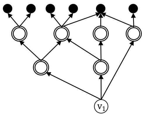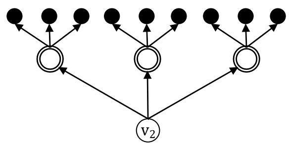 Figure 3: A fault network comprised of two disconnected components. Each component has one root node ## iii. Decentralized FPR Sequencer Maximizing Preventability: FPR-DP The FPR sequencer maximizing $P$ (FPR-DP) aims to maximize $P$ for a fault network. The FPR-DP guarantees that $P$ is maximized for a fault network comprised of disconnected components, each of which has one leaf node (LEMMA 2). In Figure 4, $v_{1}, v_{2}, v_{3}$, and $v_{4}$ should be repaired before $v_{5}, v_{6}, v_{7}, v_{8}, v_{9}$, and $v_{10}$. Faults in many complex systems may be prevented. For example, most nodes become faulty almost instantaneously when a smart grid experiences a cascading failure. Some leaf nodes have backup power supply and may sustain operations for a certain period of time. Faults at these nodes may be prevented if root nodes are repaired before the backup power runs out. ### The FPR-DP sequencer: Step 1: Select a leaf node $v_{l}$, at which faults have not occurred, such that $n_{l} \leq n_{l'}$ for $\forall v_{l'}$; faults at $v_{l'}$ have not occurred. $n_{l}$ and $n_{l'}$ are the number of root nodes $v_{r}$ 's and $v_{r'}$ 's, respectively, from which there exists at least one path to $v_{l}$ and $v_{l'}$, respectively. Randomly select a leaf node $v_{l}$ if there are multiple $v_{l}$ 's with the same $n_{l}$; Step 2: Repair all $n_l v_r$ 's; Step 3: Go to Step 1 if not all $v_{l}$ 's are prevented; otherwise go to Step 4; Step 5: Randomly select a root node $v_{r}$; $v_{r}$ has not been repaired; Step 6: Compare the required repair resources for $v_r$ and available repair resources; If the required repair resources $\leq$ available repair resources Step 7: Repair $\boldsymbol{v}_r$ Else Step 6: Go to Step 4; Step 7: Go to Step 4 if not all $v_r$ 's are repaired or are being repaired; otherwise stop. LEMMA 2: In a fault network $G(V^{F}, A^{F})$, all $n_{l}v_{r}$ 's shall be selected for repair to maximize $P$ if there exists at least one path from $v_{r}$ to $v_{l}$ and $n_{l} \leq n_{l'}$ for $\forall v_{l'}$; faults at $v_{l}$ and $v_{l'}$ have not occurred. $G(V^{F}, A^{F})$ meets three conditions: (a) for $\forall v_{r}$, except the orphan nodes, there is only one $v_{l}$ such that there exists at least one path from $v_{r}$ to $v_{l}$; (b) $t_{l} \approx t_{l'}$ for $\forall v_{l / l'}$; and (c) $m_{r} \approx m_{r'}$ for $v_{r / r'}$. Proof: Let $v_{l}$ and $v_{l^{\prime}}$ represent two leaf nodes in a fault network $G(V^{F}, A^{F})$. Faults at $v_{l}$ and $v_{l^{\prime}}$ have not occurred and may be prevented. $v_{l}$ is caused by total $n_{l}$ root nodes $v_{r}$ 's, $n_{l} > 0$; there exists at least one path from any $v_{r}$ to $v_{l}$. $v_{l}$ is repaired or prevented if and only if all $n_{l}v_{r}$ 's are repaired. Any $v_{r}$ does not cause faults at other leaf nodes other than $v_{l}$. Similarly, $v_{l^{\prime}}$ is caused by total $n_{l^{\prime}}$ root nodes $v_{r^{\prime}}$ 's, $n_{l^{\prime}} > 0$; there exists at least one path from any $v_{r^{\prime}}$ to $v_{l^{\prime}}$. Any $v_{r^{\prime}}$ does not cause faults at other leaf nodes other than $v_{l^{\prime}}$. Repairing root nodes can prevent faults at leaf nodes from occurring. Assume that $t_{l} \approx t_{l^{\prime}} > 0$, i.e., faults at leaf nodes occur at the same time, and $m_{r} \approx m_{r^{\prime}} > 0$, i.e., repair time for any root node is the same. Without losing generality, assume that $n_{l} \leq n_{l^{\prime}}$. Therefore $m_{r}n_{l} \leq m_{r^{\prime}}n_{l^{\prime}}$. $m_{r}n_{l}$ is the minimum required time to repair or prevent faults at $v_{l}$. $m_{r^{\prime}}n_{l^{\prime}}$ is the minimum required time to repair or prevent faults at $v_{l^{\prime}}$. $t_{0}$ is the time at which the FPR sequence begins repairs; $t_{0} \geq t_{r}$ and $t_{0} \geq t_{r^{\prime}}$. The time at which faults at the leaf nodes occur, $t_{l}$ or $t_{l^{\prime}}$, falls into four intervals: $t_{l / l^{\prime}} < m_{r}n_{l} + t_{0}$, $m_{r}n_{l} + t_{0} \leq t_{l / l^{\prime}} < m_{r^{\prime}}n_{l^{\prime}} + t_{0}$, $m_{r^{\prime}}n_{l^{\prime}} + t_{0} \leq t_{l / l^{\prime}} < m_{r}n_{l} + m_{r^{\prime}}n_{l^{\prime}} + t_{0}$, and $t_{l / l^{\prime}} \geq m_{r}n_{l} + m_{r^{\prime}}n_{l^{\prime}} + t_{0}$. If $t_{l / l'} < m_r n_l + t_0$, $t_{l / l'} < m_{r'} n_{l'} + t_0$ because $m_r n_l \leq m_{r'} n_{l'}$. Neither $v_l$ nor $v_{l'}$ can be prevented. $P = 0$. If $m_r n_l + t_0 \leq t_{l / l'} < m_{r'} n_{l'} + t_0$, $v_{l'}$ cannot be prevented. To maximize $P$, $v_r$ 's are repaired before the repair of $v_{r'}$ 's. $P = \frac{1}{|V^F|}$ if all $n_l v_r$ 's are repaired. $P = 0$ if $v_{r'}$ 's are repaired first or a mix of $v_r$ 's and $v_{r'}$ 's are repaired such that not all $n_l v_r$ 's are repaired by $t_{l / l'}$. If $m_{r'} n_{l'} + t_0 \leq t_{l / l'} < m_r n_l + m_{r'} n_{l'} + t_0$, either $v_l$ or $v_{l'}$ This completes the proof of LEMMA 2. can be prevented, but not both. $P = \frac{1}{|V^F|}$ if all $n_l v_r$'s are repaired first or all $n_l' v_{r'}$'s are repaired first. $P = 0$ if a mix of $v_r$'s and $v_{r'}$'s are repaired; not all $n_l v_r$'s are repaired by time $t_{l/l'}$ and neither are $n_l' v_{r'}$'s. If $t_{l/l'} \geq m_r n_l + m_{r'} n_{l'} + t_0$, both $v_l$ and $v_{l'}$ are prevented and $P = \frac{2}{|V^F|}$ regardless of the FPR sequence. In summary, repairing all $n_l v_r$'s first always maximizes $P$.  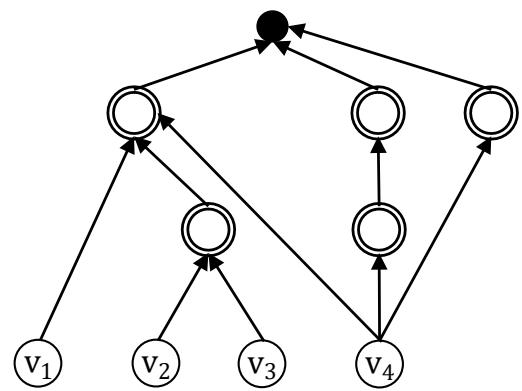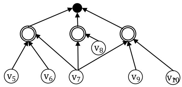 Figure 4: A fault network comprised of two disconnected components. Each component has one leaf node ## V. RESULTS To compare and validate the FPR sequencers, Monte-Carlo simulation experiments (Nasiruzzaman et al., 2014) are designed and conducted using AutoMod (Applied Materials, 1988-2009). Many real-world complex systems may not satisfy conditions in LEMMA 1 or LEMMA 2. The objectives of the experiments are to examine whether (a) the FPR-C results in the highest total damage $D$ and lowest preventability $P$; (b) the FPR-DD minimizes $D$; (c) the FPR-DP maximizes $P$; and (d) the FPR-DR performs better than the FPR-C but worse than the FPR-DD and FPR-PP. Whether the FPR-DD can minimize $D$ and the FPR-DP can maximize $P$ depend on conditions in LEMMA 1 and LEMMA 2. In LEMMA 1, it is assumed that (a) each leaf node, except the orphan node, has only one root node; (b) nodes become faulty at almost the same time; (c) damage caused by failures at each leaf node is approximately the same; and (d) repair resources, e.g., repair personnel, required for each root node is approximately the same. In LEMMA 2, it is assumed that (a) each root node, except the orphan node, has only one leaf node; (b) all leaf nodes become faulty at almost the same time; and (c) repair resources, e.g., repair personnel required for each root node are approximately the same. The structure of a fault network is derived from the structure of a complex system, and rarely satisfies condition (a) in either LEMMA 1 or LEMMA 2. In general, a root node may have multiple leaf nodes and a leaf node may have multiple root nodes. Condition (b) in LEMMA 1 and LEMMA 2 specifies the type of failures in a complex system. Three types of failures, random, cascading, and cascading with backup capacity, are studied in the experiments. Most random failures are independent of each other and occur over a long period of time. Random failures do not satisfy condition (b) in either LEMMA 1 or LEMMA 2. A cascading failure in a complex system (Nedic et al., 2006) occurs in a relatively short period of time and includes multiple faults most of which are caused by a few faulty sources (root nodes in a fault network; Hoffmann and Payton, 2014). A cascading failure satisfies condition (b) because nodes become faulty almost at the same time. A cascading failure with backup capacity does not satisfy condition (b) since leaf nodes become faulty at different times depending on the amount of backup capacity each leaf node has. Conditions (c) and (d) in LEMMA 1 and condition (c) in LEMMA 2 are valid for many complex systems. A fault network's properties along the four conditions in LEMMA 1 and LEMMA 2 determine the structure of the fault network. In each experiment, a fault network is first generated; an FPR sequencer is used to generate an FPR sequence, which is emulated to prevent and repair faults. $D$ and $P$ are calculated for each experiment. The experiments use the electrical power grid of the Western United States (Watts and Strogatz, 1998), which has 4,941 nodes, including generators, transformers, and substations. In a simulation experiment, each node has 0.1 probability of becoming faulty. Resources required to repair failures at a root node are assumed to be randomly and uniformly distributed between 3 and 10 units. For example, to repair faults at a node may require a crew of 6 people, i.e., 6 units of resources. The damage per second caused by faults at a node is randomly and uniformly distributed between $5 and$ 15. Each simulation experiment emulates an FPR sequence for 24 hours. Total repair resources affect the performance of FPR sequencers. The FPR-C repairs one root node at a time. Since the maximum amount of resources needed to repair a root node is 10 units, total repair resources for the FPR-C are 10 units, which are sufficient for the repair of any root node. The decentralized FPR sequencers, FPR-DD, FPR-DP, and FPR-DR repair multiple root nodes at the same time. The electrical power grid of the Western United States has 4,941 nodes and each node has 0.1 probability of having faults in the experiments. There are on average 494 nodes that become faulty in an experiment. Since only root nodes, including orphan nodes that are both root and leaf nodes, require repair, different levels of total repair resources are applied in the experiments according to the number of root nodes. ### a) Random Failures Many complex systems have random failures most of which occur independent of each other. In the simulation experiments, the time at which random failures occur is uniformly distributed between 0 and 86,400 seconds (24 hours = 86,400 seconds). One-hundred experiments are conducted for each combination of an FPR sequencer and a certain amount of total repair resources, which are 10 units for the FPR-C. It is necessary to determine the maximum required total repair resources (MRT), which is the amount of resources sufficient to repair all root nodes simultaneously. The simulation experiments show that the maximum number of root nodes with random failures is 523, with a mean of 464 and a standard deviation of 19. Since a root node requires at most 10 units to repair, the MRT for random failures is about 5,000 units. For scalability evaluation, 14 levels of total repair resources are used in the experiments for each of the FPR-DD, FPR-DP, and FPR-DR: 10, 50, 100, 200, 300, 400, 500, 1,000, 1,500, 2,000, 2,500, 5,000, 7,500, and 10,000 units. A decentralized FPR sequencer is expected to have the best performance when total repair resources are at or greater than the MRT. The two levels, 7,500 and 10,000 units, are included in the experiments to validate the best performance of an FPR sequencer. Total 4,300 experiments (100 experiments for FPR-C plus three decentralized FPR sequencers times 14 levels of total repair resources times 100 experiments) are conducted to compare and validate the performance of FPR sequencers for random failures. Figures 5-15 and Table 3 summarize experiment results, which provide several important findings for managing random failures: - (a) All decentralized FPR sequencers perform better than the FPR-C, which is a centralized FPR sequencer and has the maximum $D$ and minimum $P$. At the same level of total repair resources, 10 units, all three decentralized FPR sequencers significantly decrease $D$ and increase $P$ compared to the FPR-C. Because Monte-Carlo simulation allows for sampling of the entire population with 100 experiments for each combination of the FPR sequencer and level of total available repair resources, statistically significant tests are not necessary, and the difference shown in Figures 5-15 is the actual difference between the FPR sequencers; - (b) Decentralized FPR sequencers have the best performance, i.e., minimum $D$ and maximum $P$, when total repair resources are at least the MRT. Note that the upper limit for $P$ is the percentage of leaf nodes in a fault network. The experiments show that the mean and standard deviation of the percentage of leaf nodes are 0.05990 and 0.01088, respectively. The mean 0.05990 is just slightly greater than the mean for $P$ once the performance levels off; - (c) The performance of decentralized FPR sequencers first improves as total repair resources increase, and then reaches the best performance and levels off; - (d) For total damage $D$, the performance of decentralized FPR sequencers levels off once repair resources reach 200 units. In other words, if total repair resources are sufficient to repair on average $6.63\%$ ( $\approx 200 / 6.5 / 464$ ) of all root nodes, increasing the level of repair resources further does not affect the mean or standard deviation of $D$; - (e) For preventability $P$, the performance of decentralized FPR sequencers levels off once repair resources reach 100 units. In other words, if total available repair resources are sufficient to repair on average $3.32\%$ ( $\approx 100/6.5/464$ ) of all root nodes, increasing the level of repair resources further does not affect the mean or standard deviation of $P$; and - (f) The FPR-DD and FPR-DP perform almost the same, and better than the FPR-DR before the performance levels off. This experiment finding validates LEMMA 1 and LEMMA 2. In summary, either the FPR-DD or FPR-DP should be used to sequence repairs of random failures in a complex system. Increasing total repair resources up to the amount that is sufficient to repair on average $3.32\%$ of all root causes prevents more faults from occurring. After the amount is reached, further increasing total repair resources does not increase the number of faults prevented. Increasing total repair resources up to the amount that is sufficient to repair on average $6.63\%$ of all root causes decreases total damage caused by faults. After the amount is reached, further increasing total repair resources does not decrease total damage.  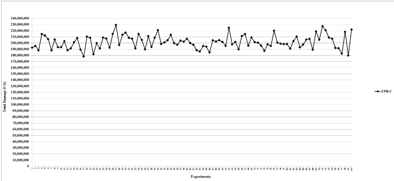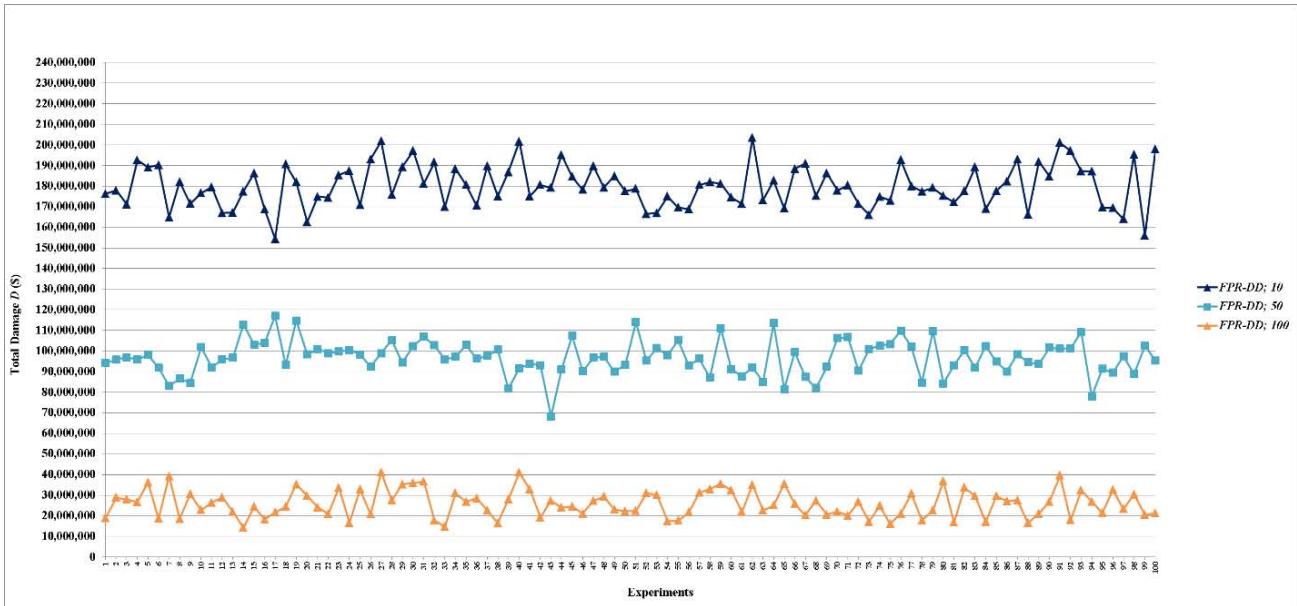 Figure 5: Total damage $D$ of fault networks with random failures using the FPR-C 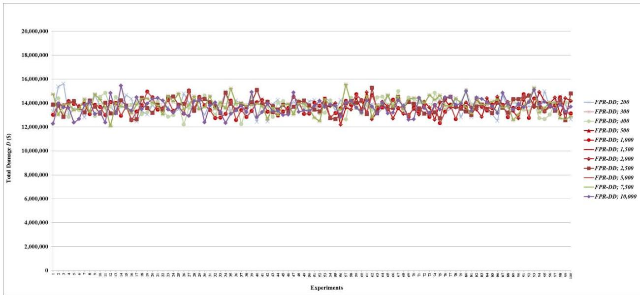 Figure 6: Total damage $D$ of fault networks with random failures using the FPR-DD with resources 10, 50, and 100 units 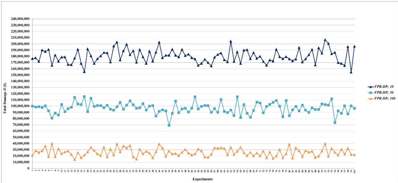 Figure 7: Total damage $D$ of fault networks with random failures using the FPR-DD with resources 200, 300, 400, 500, 1,000, 1,500, 2,000, 2,500, 5,000, 7,500, and 10,000 units 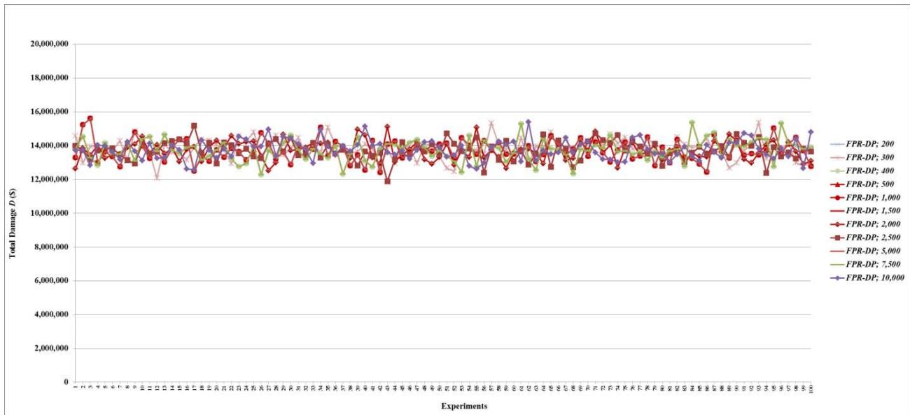 Figure 8: Total damage $D$ of fault networks with random failures using the FPR-DP with resources 10, 50, and 100 units 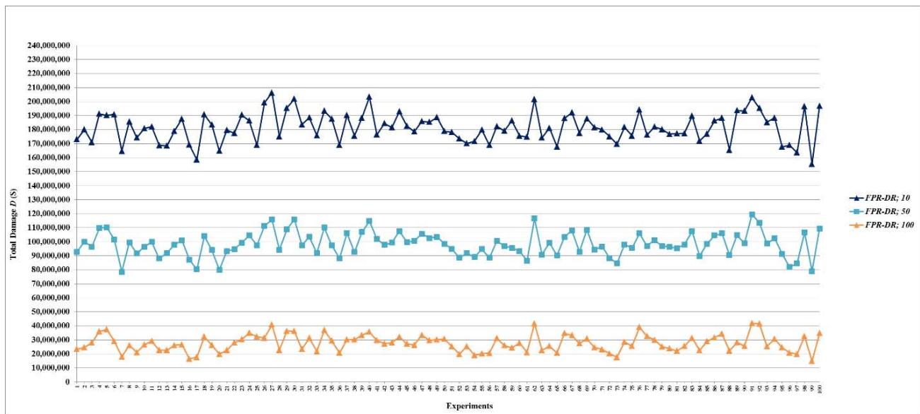 Figure 9: Total damage $D$ of fault networks with random failures using the FPR-DP with resources 200, 300, 400, 500, 1,000, 1,500, 2,000, 2,500, 5,000, 7,500, and 10,000 units 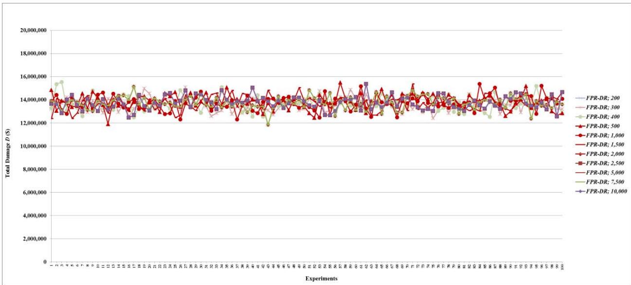 Figure 11: Total damage $D$ of fault networks with random failures using the FPR-DR with resources 200, 300, 400, 500, 1,000, 1,500, 2,000, 2,500, 5,000, 7,500, and 10,000 units 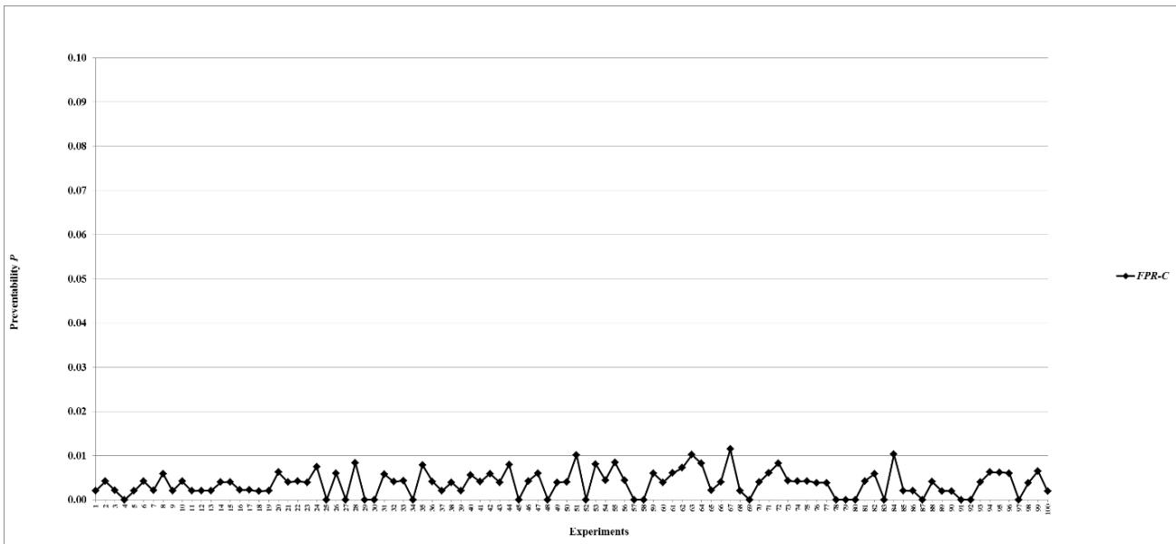 Figure 12: Preventability $P$ of fault networks with random failures using the FPR-C  Figure 10: Total damage $D$ of fault networks with random failures using the FPR-DR with resources 10, 50, and 100 units 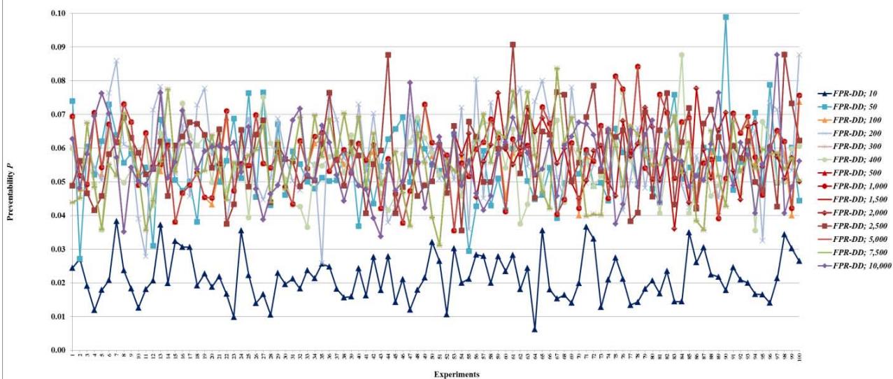 Figure 13: Preventability $P$ of fault networks with random failures using the FPR-DD 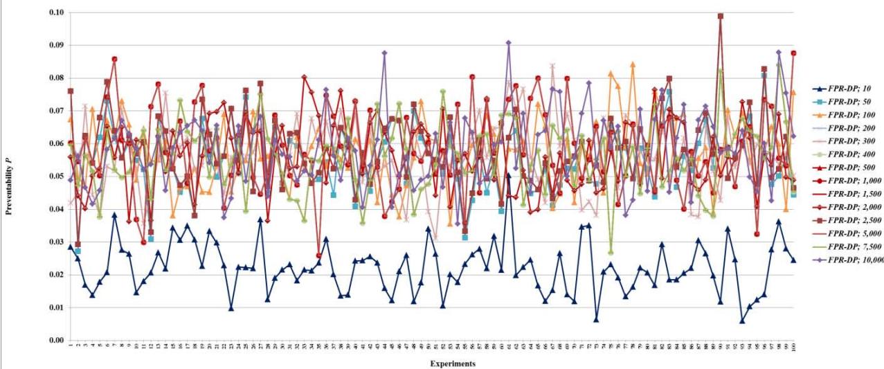 Figure 14: Preventability $P$ of fault networks with random failures using the FPR-DP 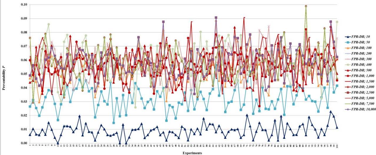 Figure 15: Preventability $P$ of fault networks with random failures using the FPR-DR Table 3: Total Damage and Preventability of Fault Networks with Random Failures <table><tr><td rowspan="2">FPR Sequencer; Total Available Repair Resources</td><td colspan="2">Total Damage D</td><td colspan="2">Preventability P</td></tr><tr><td>Mean</td><td>Standard Deviation</td><td>Mean</td><td>Standard Deviation</td></tr><tr><td>FPR-C</td><td>201621025</td><td>10828850</td><td>0.00374</td><td>0.00280</td></tr><tr><td></td><td></td><td></td><td></td><td></td></tr><tr><td>FPR-DD; 10</td><td>180006159</td><td>10313564</td><td>0.02169</td><td>0.00679</td></tr><tr><td>FPR-DD; 50</td><td>96732479</td><td>8447916</td><td>0.05502</td><td>0.01098</td></tr><tr><td>FPR-DD; 100</td><td>25934287</td><td>6586766</td><td>0.05713</td><td>0.01023</td></tr><tr><td>FPR-DD; 200</td><td>13735920</td><td>619541</td><td>0.05819</td><td>0.01251</td></tr><tr><td>FPR-DD; 300</td><td>13830873</td><td>627624</td><td>0.05627</td><td>0.01033</td></tr><tr><td>FPR-DD; 400</td><td>13717879</td><td>584635</td><td>0.05566</td><td>0.00952</td></tr><tr><td>FPR-DD; 500</td><td>13758247</td><td>569952</td><td>0.05815</td><td>0.01138</td></tr><tr><td>FPR-DD; 1,000</td><td>13630487</td><td>570632</td><td>0.05748</td><td>0.01032</td></tr><tr><td>FPR-DD; 1,500</td><td>13830873</td><td>627624</td><td>0.05627</td><td>0.01033</td></tr><tr><td>FPR-DD; 2,000</td><td>13630578</td><td>666306</td><td>0.05704</td><td>0.00973</td></tr><tr><td>FPR-DD; 2,500</td><td>13758247</td><td>569952</td><td>0.05815</td><td>0.01138</td></tr><tr><td>FPR-DD; 5,000</td><td>13630487</td><td>570632</td><td>0.05748</td><td>0.01032</td></tr><tr><td>FPR-DD; 7,500</td><td>13830873</td><td>627624</td><td>0.05627</td><td>0.01033</td></tr><tr><td>FPR-DD; 10,000</td><td>13675877</td><td>643748</td><td>0.05621</td><td>0.01009</td></tr><tr><td></td><td></td><td></td><td></td><td></td></tr><tr><td>FPR-DP; 10</td><td>180111362</td><td>10611192</td><td>0.02233</td><td>0.00769</td></tr><tr><td>FPR-DP; 50</td><td>96873761</td><td>8561127</td><td>0.05538</td><td>0.01104</td></tr><tr><td>FPR-DP; 100</td><td>25867769</td><td>6277847</td><td>0.05707</td><td>0.01032</td></tr><tr><td>FPR-DP; 200</td><td>13722287</td><td>621941</td><td>0.05825</td><td>0.01248</td></tr><tr><td>FPR-DP; 300</td><td>13833200</td><td>617975</td><td>0.05622</td><td>0.01042</td></tr><tr><td>FPR-DP; 400</td><td>13739117</td><td>637874</td><td>0.05608</td><td>0.01044</td></tr><tr><td>FPR-DP; 500</td><td>13725355</td><td>561576</td><td>0.05768</td><td>0.01126</td></tr><tr><td>FPR-DP; 1,000</td><td>13720615</td><td>621869</td><td>0.05823</td><td>0.01248</td></tr><tr><td>FPR-DP; 1,500</td><td>13739117</td><td>637874</td><td>0.05608</td><td>0.01044</td></tr><tr><td>FPR-DP; 2,000</td><td>13714074</td><td>564894</td><td>0.05680</td><td>0.01039</td></tr><tr><td>FPR-DP; 2,500</td><td>13725355</td><td>561576</td><td>0.05768</td><td>0.01126</td></tr><tr><td>FPR-DP; 5,000</td><td>13720615</td><td>621869</td><td>0.05823</td><td>0.01248</td></tr><tr><td>FPR-DP; 7,500</td><td>13739117</td><td>637874</td><td>0.05608</td><td>0.01044</td></tr><tr><td>FPR-DP; 10,000</td><td>13760036</td><td>581581</td><td>0.05815</td><td>0.01138</td></tr><tr><td></td><td></td><td></td><td></td><td></td></tr><tr><td>FPR-DR; 10</td><td>181502337</td><td>10358006</td><td>0.00916</td><td>0.00472</td></tr><tr><td>FPR-DR; 50</td><td>98257539</td><td>8680622</td><td>0.03252</td><td>0.00845</td></tr><tr><td>FPR-DR; 100</td><td>27572124</td><td>5995100</td><td>0.05421</td><td>0.01164</td></tr><tr><td>FPR-DR; 200</td><td>13731751</td><td>557508</td><td>0.05774</td><td>0.01137</td></tr><tr><td>FPR-DR; 300</td><td>13619331</td><td>566126</td><td>0.05734</td><td>0.01029</td></tr><tr><td>FPR-DR; 400</td><td>13719841</td><td>626493</td><td>0.05817</td><td>0.01243</td></tr><tr><td>FPR-DR; 500</td><td>13834270</td><td>626768</td><td>0.05635</td><td>0.01046</td></tr><tr><td>FPR-DR; 1,000</td><td>13730883</td><td>634684</td><td>0.05610</td><td>0.01047</td></tr><tr><td>FPR-DR; 1,500</td><td>13712596</td><td>590669</td><td>0.05815</td><td>0.01120</td></tr><tr><td>FPR-DR; 2,000</td><td>13730156</td><td>556901</td><td>0.05774</td><td>0.45707</td></tr><tr><td>FPR-DR; 2,500</td><td>13743341</td><td>577436</td><td>0.05832</td><td>0.01131</td></tr><tr><td>FPR-DR; 5,000</td><td>13730156</td><td>556901</td><td>0.05774</td><td>0.01137</td></tr><tr><td>FPR-DR; 7,500</td><td>13730156</td><td>556901</td><td>0.05774</td><td>0.01137</td></tr><tr><td>FPR-DR; 10,000</td><td>13743341</td><td>577436</td><td>0.05832</td><td>0.01131</td></tr></table> ### b) Cascading Failures A cascading failure may occur within a few minutes to a few hours (Andersson et al., 2005). For example, significant failures in the U.S.-Canadian blackout of August 14, 2003, occurred in less than an hour. In the simulation experiments, the time at which faults as part of a cascading failure occur is uniformly and randomly distributed between 42,300 and 44,100 seconds $(43,200 \pm 900)$, i.e., faults occur within 30 minutes. The simulation experiments show that the maximum number of root nodes is 94 with a mean of 66 and a standard deviation of 9. Since a root node requires at most 10 units to repair, the MRT for a cascading failure is about 1,000 units. For scalability evaluation, 10 levels of total repair resources are used in the experiments for each of the FPR-DD, FPR-DP, and FPR-DR: 10, 50, 100, 200, 300, 400, 500, 1,000, 1,500, and 2,000 units. Total 3,100 experiments (100 experiments for FPR-C plus three decentralized FPR sequencers times 10 levels of total repair resources times 100 experiments) are conducted to compare and validate the performance of FPR sequencers for cascading failures. Figures 16-22 and Table 4 summarize experiment results, which provide several important findings for managing cascading failures: - (a) The preventability $P$ of all FPR sequencers is zero. This is often the case in a complex system where a cascading failure occurs in a short period of time, and no faults may be prevented once the cascading failure begins unfolding; - (b) All decentralized FPR sequencers have smaller $D$ than the FPR-C with the same amount of total repair resources; - (c) Decentralized FPR sequencers have the minimum $D$ when total repair resources are at least the MRT; - (d) Decentralized FPR sequencers first decrease $D$ as total repair resources increase, and then reaches the minimum $D$, which levels off once repair resources reach 500 units. In other words, if total repair resources are sufficient to repair on average $100\%$ ( $\approx$ 500/6.5/66) of all root nodes in a cascading failure, increasing the level of repair resources further does not affect the mean or standard deviation of $D$; and (e) The FPR-DD and FPR-DP have almost the same $D$, which is less than that of the FPR-DR before $D$ levels off. This experiment finding validates LEMMA 1 and LEMMA 2. In summary, either the FPR-DD or FPR-DP should be used to sequence repairs of a cascading failure in a complex system. Increasing total repair resources up to the amount that is sufficient to repair all root nodes decreases total damage caused by faults. After the amount is reached, further increasing total repair resources does not reduce total damage. Compared to random failures, a cascading failure has less damage with the same level of total repair resources. This is because most faults in a cascading failure are caused by a few root nodes (with a mean of 66) whereas most faults in random failures are root nodes (with a mean of 464) and require repairs. In the simulation experiments, it is assumed that approximately the same number of faults (with a mean of 494) occur in random failures within 24 hours and in a cascading failure within 30 minutes. In real-world complex systems, however, these faults in random failures may occur across a much longer time period, for instance, two to three years. Total damage caused by random failures is greater but over a more extended period. 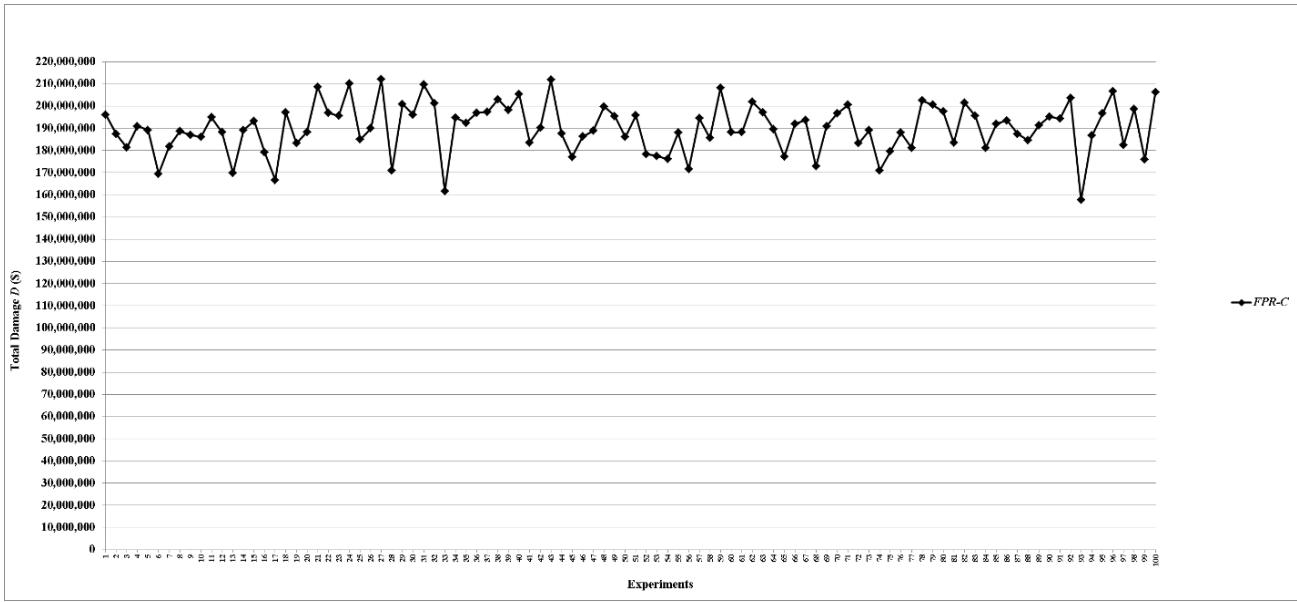 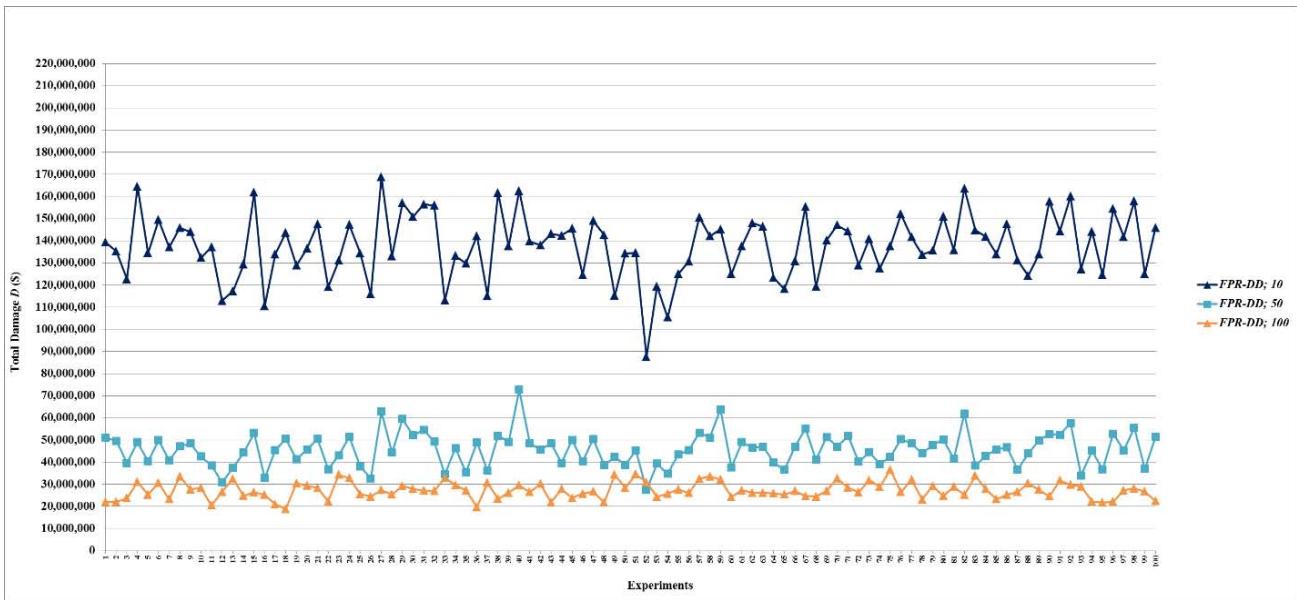Figure 16: Total damage $D$ of fault networks with cascading failures using the FPR-C  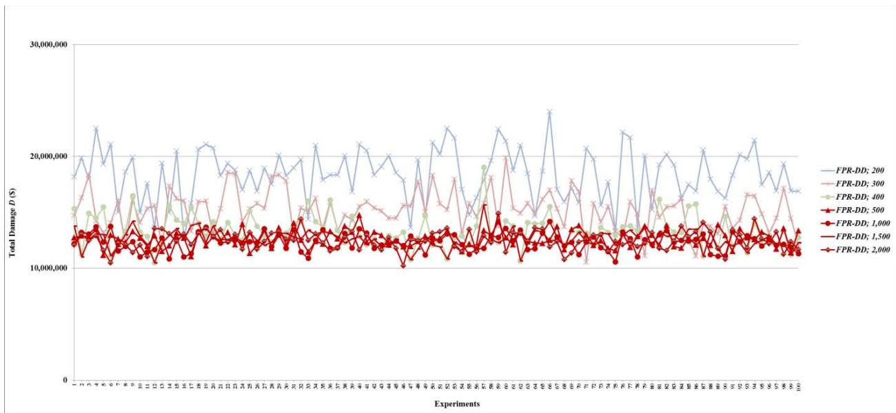 Figure 17: Total damage $D$ of fault networks with cascading failures using the FPR-DD with resources 10, 50, and 100 units 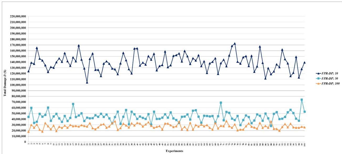 Figure 18: Total damage $D$ of fault networks with cascading failures using the FPR-DD with resources 200, 300, 400, 500, 1,000, 1,500, and 2,000 units 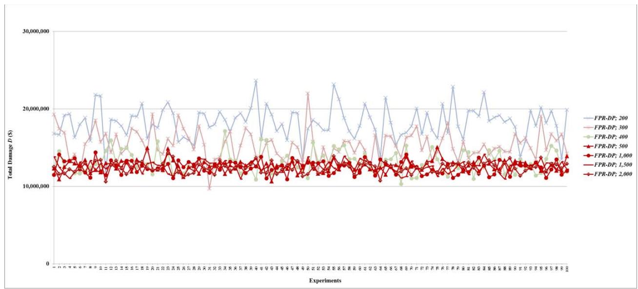 Figure 19: Total damage $D$ of fault networks with cascading failures using the FPR-DP with resources 10, 50, and 100 units 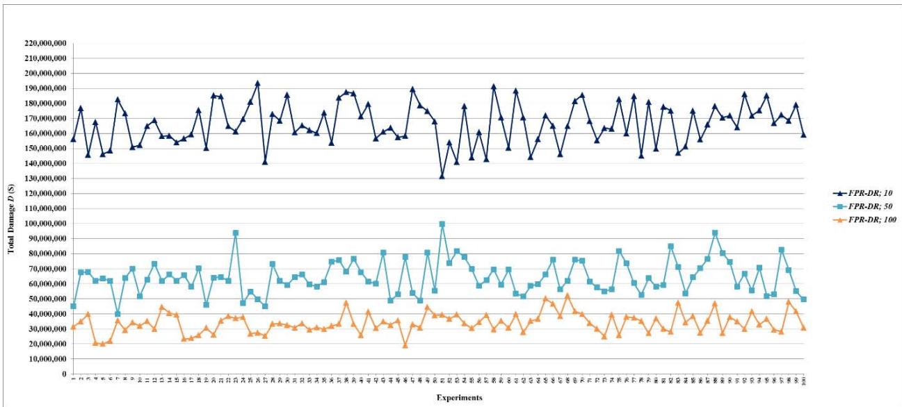 Figure 20: Total damage $D$ of fault networks with cascading failures using the FPR-DP with resources 200, 300, 400, 500, 1,000, 1,500, and 2,000 units 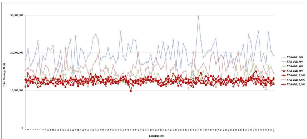 Figure 21: Total damage $D$ of fault networks with cascading failures using the FPR-DR with resources 10, 50, and 100 units Table 4: Total Damage and Preventability of Fault Networks with Cascading Failures <table><tr><td rowspan="2">FPR Sequencer; Total Available Repair Resources</td><td colspan="2">Total Damage D</td><td colspan="2">Preventability P</td></tr><tr><td>Mean</td><td>Standard Deviation</td><td>Mean</td><td>Standard Deviation</td></tr><tr><td>FPR-C</td><td>190139716</td><td>11025184</td><td>0</td><td>0</td></tr><tr><td></td><td></td><td></td><td></td><td></td></tr><tr><td>FPR-DD; 10</td><td>137672499</td><td>14383251</td><td rowspan="10">0</td><td rowspan="10">0</td></tr><tr><td>FPR-DP; 50</td><td>44591923</td><td>8105005</td></tr><tr><td>FPR-DP; 100</td><td>27451992</td><td>4244597</td></tr><tr><td>FPR-DP; 200</td><td>18238043</td><td>2105204</td></tr><tr><td>FPR-DP; 300</td><td>15364209</td><td>1846987</td></tr><tr><td>FPR-DP; 400</td><td>130</td></tr></table>  Figure 22: Total damage $D$ of fault networks with cascading failures using the FPR-DR with resources 200, 300, 400, 500, 1,000, 1,500, and 2,000 units  ### 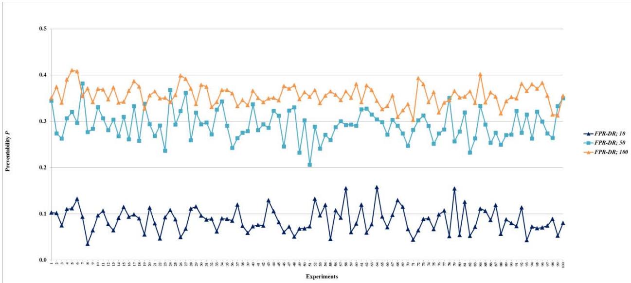c) Cascading Failures with Backup Capacity Many critical nodes in a complex system have backup capacity in case of failures. For example, consumers in a smart grid can have backup power that provides uninterrupted power supply when there is a random failure or a cascading failure. Backup power may be fueled by gasoline, diesel, propane, natural gas, battery, and other energy sources. Some provide protection against failures and others require a short period of time, for example, 30 seconds, to resume power supply. Backup power may last for a few minutes to a few days, depending on its capacity and power usage. In theory, some generators provide an endless electricity supply using natural gas from the utility company. In practice, however, these generators require periodical maintenance, for example, replacing engine oil, or cooling. There is always a limit on how long backup power can continuously supply electricity. In the simulation experiments, the time at which root and internal nodes become faulty is uniformly and randomly distributed between 42,300 and 44,100 seconds, which is the same for root and internal nodes in a cascading failure without backup capacity (Section 5.2). The time at which leaf nodes become faulty is uniformly and randomly distributed between 46,800 and 86,400 seconds, i.e., leaf nodes with backup power become faulty approximately between 1 hour and 12 hours after their corresponding root nodes become faulty. The simulation experiments show that the maximum number of root nodes is 102, with a mean of 66 and a standard deviation of 9. Since a root node requires at most 10 units to repair, the MRT for a cascading failure with backup capacity is about 1,000 units. For scalability evaluation, 10 levels of total repair resources are used in the experiments for each of the FPR-DD, FPR-DP, and FPR-DR: 10, 50, 100, 200, 300, 400, 500, 1,000, 1,500, and 2,000 units. Total 3,100 experiments (100 experiments for FPR-C plus three decentralized FPR sequencers times 10 levels of total repair resources times 100 experiments) are conducted to compare and validate the performance of FPR sequencers for cascading failures with backup capacity. Figures 23-36 and Table 5 summarize experiment results, which provide several important findings for managing cascading failures with backup capacity: - (a) All decentralized FPR sequencers perform better than the $FPR-C$, which has the maximum $D$ and minimum $P$. At the same level of total repair resources, 10 units, all three decentralized FPR sequencers significantly decrease $D$ and increase $P$ compared to the $FPR-C$; - (b) Decentralized FPR sequencers have the best performance, i.e., minimum $D$ and maximum $P$, when total repair resources are at least the MRT. The upper limit for $P$ is the percentage of leaf nodes. The experiments show that the mean and standard deviation of the percentage of leaf nodes are 0.39720 and 0.01615, respectively. The mean 0.39720 is just slightly greater than the mean for $P$ once the performance levels off; - (c) The performance of decentralized FPR sequencers first improves as total repair resources increase, and then reaches the best performance and levels off; - (d) For total damage $D$, the performance of decentralized FPR sequencers levels off once repair resources reach 500 units. In other words, if total repair resources are sufficient to repair on average $100\%$ ( $\approx 500 / 6.5 / 66$ ) of all root nodes in a cascading failure with backup capacity, increasing the level of repair resources further does not affect the mean or standard deviation of $D$; - (e) For preventability $P$, the performance of decentralized FPR sequencers levels off once repair resources reach 300 units. In other words, if total repair resources are sufficient to repair on average $69.93\%$ ( $\approx 300 / 6.5 / 66$ ) of all root nodes in a cascading failure with backup capacity, increasing the level of repair resources further does not affect the mean or standard deviation of $P$; and - (f) The FPR-DD and FPR-DP perform almost the same, and better than the FPR-DR, before the performance levels off. This experiment finding validates LEMMA 1 and LEMMA 2. In summary, either the FPR-DD or FPR-DP should be used to sequence repairs of a cascading failure with backup capacity in a complex system. Increasing total repair resources up to the amount that is sufficient to repair on average $69.93\%$ of all root nodes prevents more faults from occurring. After the amount is reached, further increasing total repair resources does not increase the number of faults prevented. Increasing total repair resources up to the amount that is sufficient to repair $100\%$ of all root nodes decreases total damage caused by faults. After the amount is reached, further increasing total repair resources does not reduce total damage. Compared to a cascading failure without backup capacity, a cascading failure with backup capacity has lower damage with the same amount of total repair resources. The preventability of a cascading failure with backup capacity is greater than that of a cascading failure without backup capacity, which is zero regardless of the amount of repair resources. These comparison results are expected because the time that leaf nodes become faulty is delayed because of backup capacity, which reduces total damage and allows FPR sequencers to prevent more faults. Compared to random failures, a cascading failure with backup capacity has lower damage and higher preventability with the same amount of total repair resources. 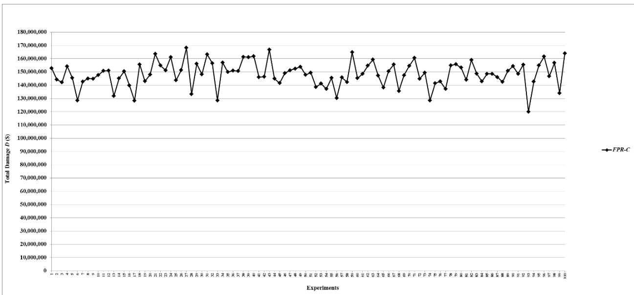 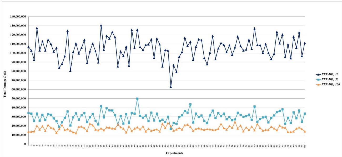Figure 23: Total damage $D$ of fault networks with cascading failures and backup capacity using the FPR-C  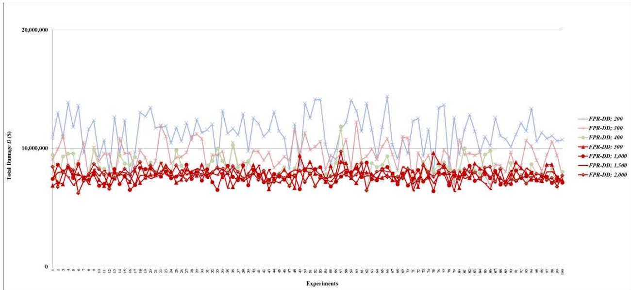 Figure 24: Total damage $D$ of fault networks with cascading failures and backup capacity using the FPR-DD with resources 10, 50, and 100 units 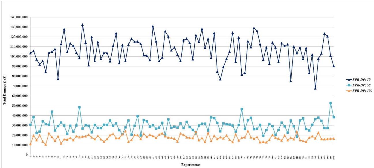 Figure 26: Total damage $D$ of fault networks with cascading failures and backup capacity using the FPR-DP with resources 10, 50, and 100 units 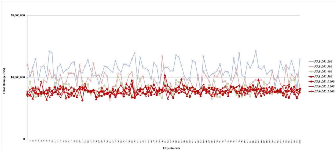 Figure 27: Total damage $D$ of fault networks with cascading failures and backup capacity using the FPR-DP with resources 200, 300, 400, 500, 1,000, 1,500, and 2,000 units 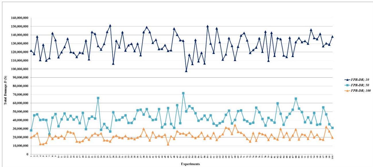 Figure 25: Total damage $D$ of fault networks with cascading failures and backup capacity using the FPR-DD with resources 200, 300, 400, 500, 1,000, 1,500, and 2,000 units 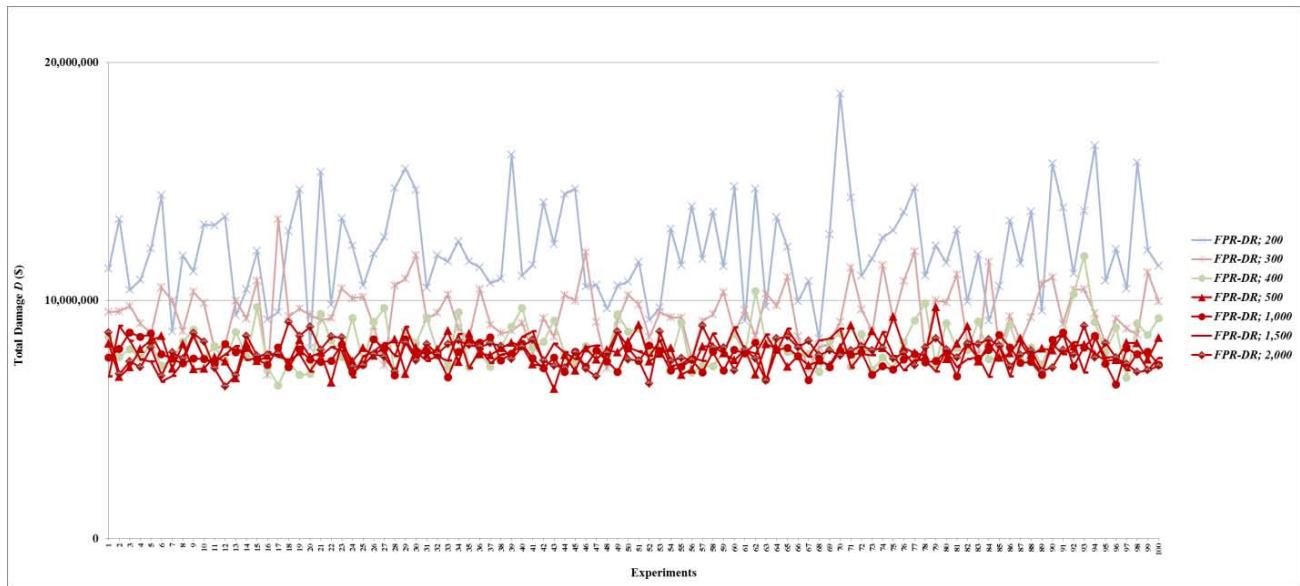 Figure 28: Total damage $D$ of fault networks with cascading failures and backup capacity using the FPR-DR with resources 10, 50, and 100 units 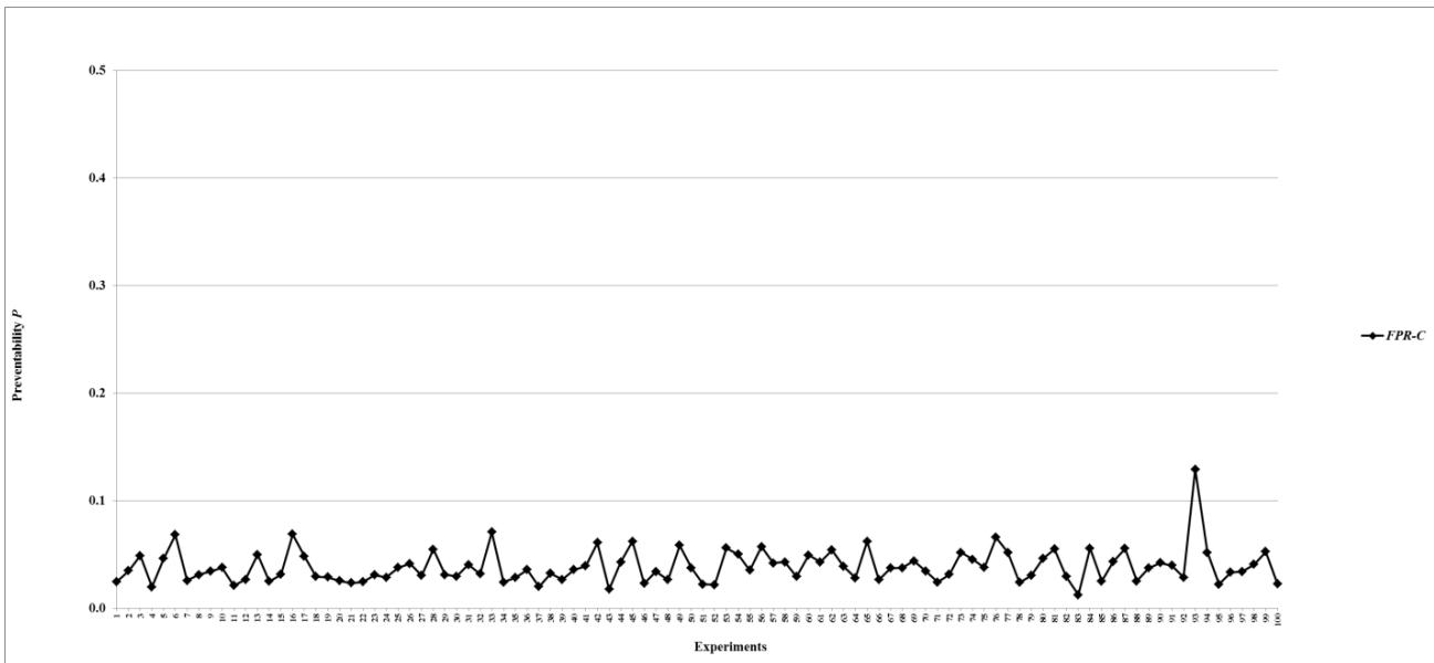 Figure 29: Total damage $D$ of fault networks with cascading failures and backup capacity using the FPR-DR with resources 200, 300, 400, 500, 1,000, 1,500, and 2,000 units 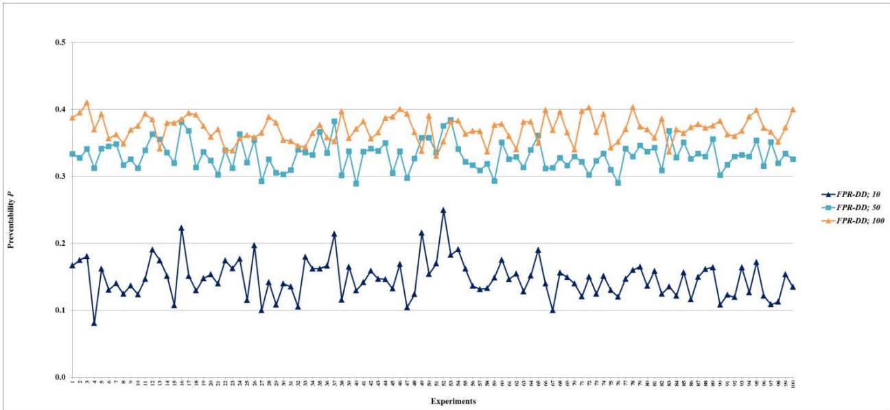 Figure 30: Preventability $P$ of fault networks with cascading failures and backup capacity using the FPR-C 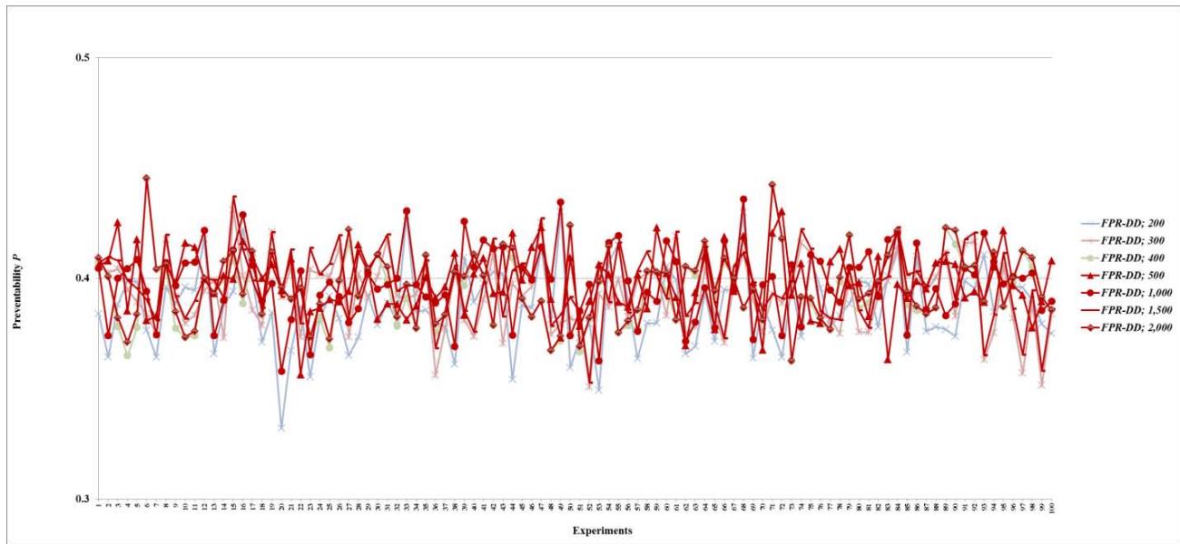 Figure 31: Preventability $P$ of fault networks with cascading failures and backup capacity using the FPR-DD with resources 10, 50, and 100 units 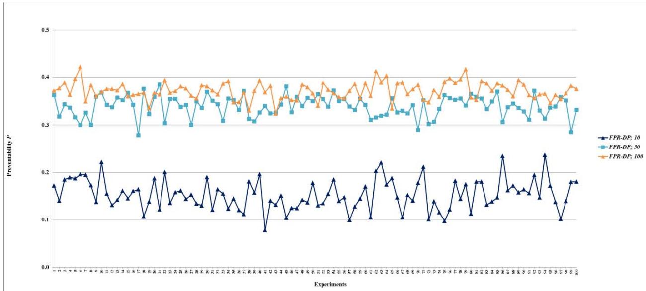 Figure 32: Preventability $P$ of fault networks with cascading failures and backup capacity using the FPR-DD with resources 200, 300, 400, 500, 1,000, 1,500, and 2,000 units Figure 33: Preventability $P$ of fault networks with cascading failures and backup capacity using the FPR-DP with resources 10, 50, and 100 units 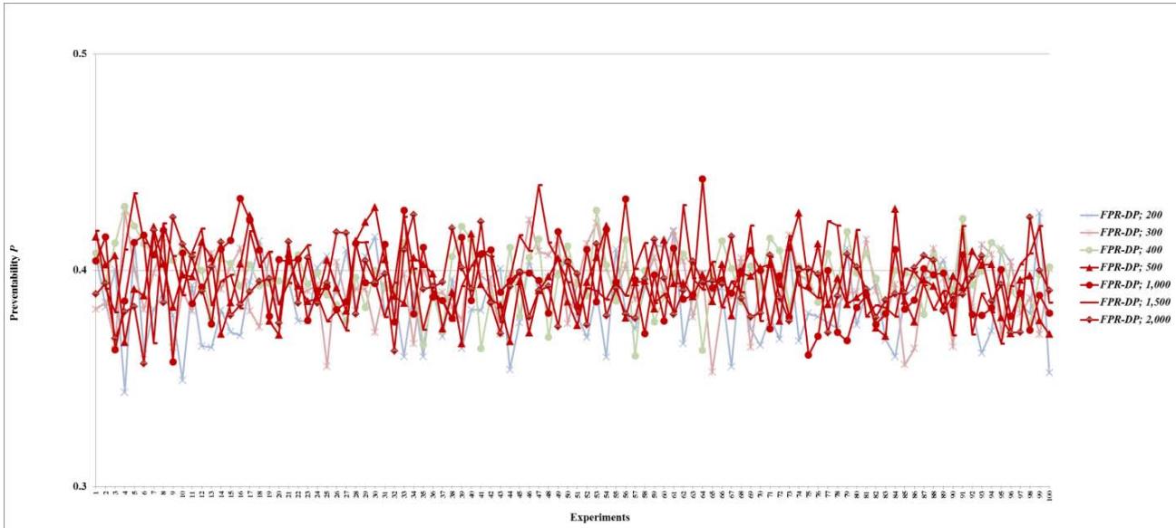 Figure 34: Preventability $P$ of fault networks with cascading failures and backup capacity using the FPR-DP with resources 200, 300, 400, 500, 1,000, 1,500, and 2,000 units  Figure 35: Preventability $P$ of fault networks with cascading failures and backup capacity using the FPR-DR with resources 10, 50, and 100 units 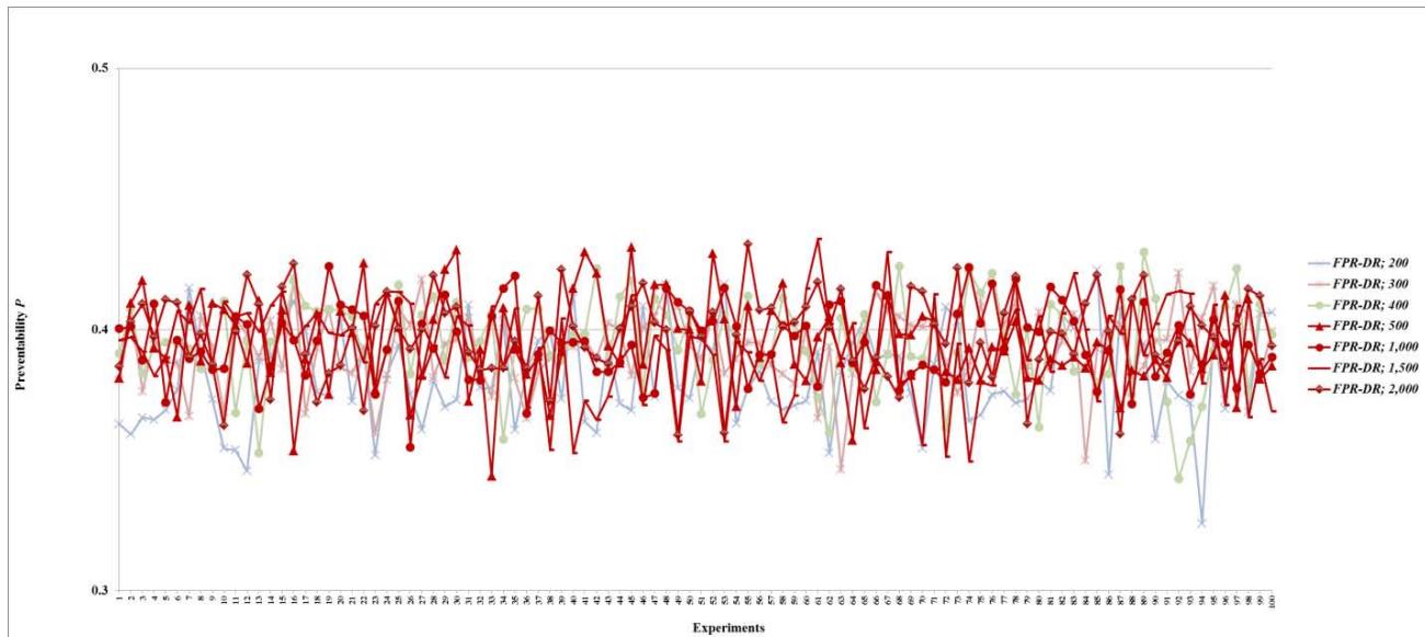 Figure 36: Preventability $P$ of fault networks with cascading failures and backup capacity using the FPR-DR with resources 200, 300, 400, 500, 1,000, 1,500, and 2,000 units Table 5: Total Damage and Preventability of Fault Networks with Cascading Failures and Backup Capacity <table><tr><td rowspan="2">FPR Sequencer; Total Available Repair Resources</td><td colspan="2">Total Damage D</td><td colspan="2">Preventability P</td></tr><tr><td>Mean</td><td>Standard Deviation</td><td>Mean</td><td>Standard Deviation</td></tr><tr><td>FPR-C</td><td>148373001</td><td>9288272</td><td>0.03851</td><td>0.01589</td></tr><tr><td></td><td></td><td></td><td></td><td></td></tr><tr><td>FPR-DD; 10</td><td>105108343</td><td>11885502</td><td>0.14739</td><td>0.02841</td></tr><tr><td>FPR-DD; 50</td><td>30052458</td><td>5563336</td><td>0.33118</td><td>0.02094</td></tr><tr><td>FPR-DD; 100</td><td>17128898</td><td>2613894</td><td>0.37075</td><td>0.01843</td></tr><tr><td>FPR-DD; 200</td><td>11367503</td><td>1570235</td><td>0.38669</td><td>0.01775</td></tr><tr><td>FPR-DD; 300</td><td>9349344</td><td>1117094</td><td>0.39201</td><td>0.01617</td></tr><tr><td>FPR-DD; 400</td><td>8254510</td><td>924284</td><td>0.39495</td><td>0.01617</td></tr><tr><td>FPR-DD; 500</td><td>7799390</td><td>604234</td><td>0.39781</td><td>0.01431</td></tr><tr><td>FPR-DD; 1,000</td><td>7636528</td><td>545318</td><td>0.39766</td><td>0.01628</td></tr><tr><td>FPR-DD; 1,500</td><td>7689905</td><td>485015</td><td>0.39747</td><td>0.01575</td></tr><tr><td>FPR-DD; 2,000</td><td>7773727</td><td>560613</td><td>0.39660</td><td>0.01593</td></tr><tr><td></td><td></td><td></td><td></td><td></td></tr><tr><td>FPR-DP; 10</td><td>105705485</td><td>13271770</td><td>0.15372</td><td>0.03176</td></tr><tr><td>FPR-DP; 50</td><td>29992260</td><td>6110029</td><td>0.33925</td><td>0.02223</td></tr><tr><td>FPR-DP; 100</td><td>17395991</td><td>2966890</td><td>0.37180</td><td>0.01803</td></tr><tr><td>FPR-DP; 200</td><td>11310111</td><td>1369366</td><td>0.38602</td><td>0.01781</td></tr><tr><td>FPR-DP; 300</td><td>9461647</td><td>855075</td><td>0.39217</td><td>0.01589</td></tr><tr><td>FPR-DP; 400</td><td>8065408</td><td>855075</td><td>0.39730</td><td>0.01407</td></tr><tr><td>FPR-DP; 500</td><td>7832061</td><td>657541</td><td>0.39407</td><td>0.01496</td></tr><tr><td>FPR-DP; 1,000</td><td>7696657</td><td>505783</td><td>0.39449</td><td>0.01668</td></tr><tr><td>FPR-DP; 1,500</td><td>7686924</td><td>512478</td><td>0.39678</td><td>0.01608</td></tr><tr><td>FPR-DP; 2,000</td><td>7830611</td><td>567063</td><td>0.39358</td><td>0.01438</td></tr><tr><td></td><td></td><td></td><td></td><td></td></tr><tr><td>FPR-DR; 10</td><td>127750386</td><td>11732134</td><td>0.08709</td><td>0.02602</td></tr><tr><td>FPR-DR; 50</td><td>42927586</td><td>8660819</td><td>0.29236</td><td>0.03252</td></tr><tr><td>FPR-DR; 100</td><td>21324304</td><td>4451081</td><td>0.35635</td><td>0.02123</td></tr><tr><td>FPR-DR; 200</td><td>12129522</td><td>2007120</td><td>0.38216</td><td>0.01887</td></tr><tr><td>FPR-DR; 300</td><td>9478993</td><td>1190272</td><td>0.39280</td><td>0.01448</td></tr><tr><td>FPR-DR; 400</td><td>8176260</td><td>924508</td><td>0.39493</td><td>0.01764</td></tr><tr><td>FPR-DR; 500</td><td>7824465</td><td>570546</td><td>0.39449</td><td>0.01706</td></tr><tr><td>FPR-DR; 1,000</td><td>7650762</td><td>487693</td><td>0.39555</td><td>0.01413</td></tr><tr><td>FPR-DR; 1,500</td><td>7761738</td><td>534957</td><td>0.39275</td><td>0.01824</td></tr><tr><td>FPR-DR; 2,000</td><td>7789133</td><td>565894</td><td>0.39807</td><td>0.03072</td></tr></table> ## VI. DISCUSSION The experiments results show that applying the FPR-DD and FPR-DP results in almost the same total damage and preventability, although the FPR-DD aims to minimize total damage and the FPR-DP aims to maximize preventability. The FPR-DD is developed based on LEMMA 1, which assumes that any fault has at most one root cause. The FPR-DP is developed based on LEMMA 2, which assumes that a root cause only causes at most one faulty leaf node. In real-world complex systems, these two assumptions are hardly accurate. A root cause may cause multiple faulty leaf nodes, whereas a faulty leaf node may be caused by multiple root causes. This many-to-many relationship is a reason why the FPR-DD and FPR-DP perform almost the same. On the other hand, both perform better than the FPR-C and FPR-DR; the latter is also a decentralized FPR sequencer that randomly selects root nodes for repairs. This finding suggests that parallelism (simultaneous repairs of multiple root nodes) and FPR sequencers that take advantage of the structure of a fault network help improve the performance of FPR sequencers. Total repair resources significantly affect the performance of FPR sequencers up to a point. Increasing repair resources improves the performance of FPR sequencers until the amount reaches a threshold. To maximize preventability requires less resource than minimizing total damage. This observation provides an important insight for managing faults in complex systems. For instance, in a transportation system with ongoing traffic problems in certain areas, a primary objective is to prevent congestion in other regions. To resolve each traffic problem as they occur may reduce damage but may not be necessary to prevent congestions elsewhere. As long as repair resources are sufficient to resolve a certain percentage of all traffic problems (69.93% if it is a cascading failure and 3.32% if traffic problems are random failures and mostly independent), any of the three decentralized FPR sequencers can prevent the maximum number of congestions from occurring. Another important insight regarding random failures is that only a small fraction of the MRT, $6.63\%$ based on the simulation experiments, is needed to minimize total damage and maximize preventability. A cascading failure may be catastrophic, but it may happen relatively rarely. Most complex systems routinely experience random failures that occur sporadically over a long period of time. The simulation experiments indicate that their long-term damage is higher than that of cascading failures, although the latter attract much more attention to the public for their broad impacts. It is not true that more repair resources always reduce damage caused by faults and prevent more faults from occurring. Random failures may be effectively and efficiently managed using the FPR-DD or FPR-DP with a relatively small amount of repair resources. ## VII. FUTURE RESEARCH The simulation experiments use the electrical power grid of the Western United States to obtain the thresholds for repair resources. Additional experiments may be conducted in the future to fine-tune the thresholds with more input from the system. Other complex systems may have different threshold values and may also be studied in the future. The simulation results also suggest that parallelism and FPR sequencers that take advantage of the structure of a fault network help improve the performance of FPR sequencers. Future research may develop other FPR sequencers and experiment with additional complex systems to further identify how different FPR sequencers perform in different systems. ## VIII. CONCLUSIONS Four fault prevention and repair sequencers, including a centralized sequencer, FPR-C, and three decentralized sequencers, FPR-DD, FPR-DP, and FPR-DR, are developed to sequence the prevention and repair of three different types of faults in a complex system, including random failures, cascading failures, and cascading failures with backup capacity. The FPR-DD aims to minimize total damage caused by faults. The FPR-DP aims to maximize preventability, the percentage of faults prevented from occurring. The FPR-DR randomly selects faults for simultaneous repairs. All four FPR sequencers are implemented in a software program to generate FPR sequences and compare and validate their performance. The electrical power grid of the Western United States is studied in total 10,500 experiments to examine the performance of the four FPR sequencers. Results show that either the FPR-DD or FPR-DP should be used to prevent and repair faults in complex systems; both sequencers minimize total damage and maximize preventability. Total repair resources affect the performance of three decentralized FPR sequencers. Total repair resources have different thresholds for different types of failures and performance metrics. Below a threshold, increasing total repair resources improves the performance of an FPR sequencer. Above the threshold, increasing total repair resources does not further improve the performance of the FPR sequencer. The threshold of repair resources is measured as a percentage of repair resources sufficient to simultaneously repair all root nodes, which are root causes and must be repaired directly using repair resources. Below is a summary of thresholds for three types of failures: - (a) Random failures: $6.63\%$ for total damage and $3.32\%$ for preventability; - (b) Cascading failures: $100\%$ for total damage. No threshold for preventability since faults are not prevented once a cascading failure begins; and - (c) Cascading failures with backup capacity: $100\%$ for total damage and $69.93\%$ for preventability. In summary, to manage a cascading failure, increasing repair resources reduces total damage caused by faults until repair resources are sufficient to repair all root causes of the cascading failure. Without backup capacity for nodes to continue operating, e.g., backup power in a smart grid, faults in a cascading failure cannot be prevented since the cascading failure happens quickly before any repair may be completed. When there is backup capacity, increasing repair resources up to $69.93\%$ of the MRT help prevent more faults from occurring. For random failures, only $6.63\%$ of the MRT are necessary to minimize total damage and $3.32\%$ of those are needed to maximize preventability. Availability of Data and Material All data used are available in this article or publicly available. Conflict of Interests None. Funding None. Authors' Contributions The author contributed $100\%$ of this article.

Generating HTML Viewer...

References

38 Cites in Article
S Alizadeh,S Sriramula (2017). Reliability modelling of redundant safety systems without automatic diagnostics incorporating common cause failures and process demand.
G Andersson,P Donalek,R Farmer,N Hatziargyriou,I Kamwa,P Kundur,N Martins,J Paserba,P Pourbeik,J Sanchez-Gasca,R Schulz,A Stankovic,C Taylor,V Vittal (2005). Causes of the 2003 major grid blackouts in North America and Europe, and recommended means to improve system dynamic performance.
C Ang (2006). Optimized Recovery of Damaged Electrical Power Grids.
Angeles Serrano,M De Los Rios,P (2007). Interfaces and the edge percolation map of random directed networks.
Li Tang,Xiaoping Qiu,Chaozhe Jiang (1988). Modeling Simulation of the Storage Management System Using AutoMod Software.
Albert-László Barabási,Réka Albert (1999). Emergence of Scaling in Random Networks.
A Barabasi (2002). Linked: The New Science of Networks.
Xin Chen,Shimon Nof (2007). PROGNOSTICS AND DIAGNOSTICS OF CONFLICTS AND ERRORS IN A SUPPLY NETWORK.
X Chen (2009). Prognostics and Diagnostics of Conflicts and Errors with Prevention and Detection Logic.
X Chen,S Nof (2010). A decentralised conflict and error detection and prediction model.
Xin Chen,Shimon Nof (2012). Conflict and error prevention and detection in complex networks.
X Chen,S Nof (2014). Interactive Conflict Detection and Resolution for Air and Air-Ground Traffic Control.
Xin Chen,Shimon Nof (2015). PROGNOSTICS AND DIAGNOSTICS OF CONFLICTS AND ERRORS IN A SUPPLY NETWORK.
Reuven Cohen,Keren Erez,Daniel Ben-Avraham,Shlomo Havlin (2000). Resilience of the Internet to Random Breakdowns.
Reuven Cohen,Keren Erez,Daniel Ben-Avraham,Shlomo Havlin (2001). Breakdown of the Internet under Intentional Attack.
M Dawande,V Mookerjeeh,C Sriskandarajah,Y Zhu (2011). Structural search and optimization in social networks.
H Dong,N Hou,Z Wang,H Liu (2019). Finite horizon fault estimation under imperfect measurements and stochastic communication protocol: Dealing with finite time boundedness.
S Dorogovtsev,J Mendes,A Samukhin (2001). Giant strongly connected component of directed networks.
Aroldo Claus,George Connolly,J Esp (2012). PDI EPRI-ENC-DMW-PA-1 Implementation Using EPRI Virtual Flaw Software - A Case of Successful Technology Transfer.
P Erdős,A Rényi (1959). On random graphs. I..
Fico (2011). Insurance Fraud Manager.
H Hoffmann,D Payton (2014). Suppressing cascades in a self-organized-critical model with non-contiguous spread of failures.
T Jin,N Mai,Y Ding,L Vo,R Dawud (2018). Planning for distribution resilience under variable generation: Prevention, surviving and recovery.
Nageswara Rao,S Viswanadham,N (1987). Fault diagnosis in dynamical systems: a graph theoretic approach.
A Nasiruzzaman,H Pota,Nahida Akter,Most (2014). Vulnerability of the large-scale future smart electric power grid.
Dusko Nedic,Ian Dobson,Daniel Kirschen,Benjamin Carreras,Vickie Lynch (2006). Criticality in a cascading failure blackout model.
M Newman,A Barabasi,D Watts (2006). The Structure and Dynamics of Networks.
S Nof,X Chen (2015). 2015 6th International Conference on the Network of the Future (NOF).
S Nof,X Chen (2017). Interactive, Constraint-Network Prognostics and Diagnostics to Control Errors and Conflicts (IPDN) Extensions.
P Parsa,X Chen (2013). Diffusion of healthy behaviors in social networks.
J Salmeron,K Wood,R Baldick (2004). Analysis of electric grid security under terrorist threat.
Teodora Sanislav,Sherali Zeadally,George Mois,Hacène Fouchal (2018). Reliability, failure detection and prevention in cyber‐physical systems (CPSs) with agents.
S Sim,J Endrenyi (1993). Failure-repair model with minimal and major maintenance.
Ray Solomonoff,Anatol Rapoport (1951). Connectivity of random nets.
Duncan Watts,Steven Strogatz (1998). Collective dynamics of ‘small-world’ networks.
L Zou,Z Wang,J Hu,Y Liu,X Liu (2021). Communication-protocol-based analysis and synthesis of networked systems: progress, prospects and challenges.
No ethics committee approval was required for this article type.
Data Availability
Not applicable for this article.
How to Cite This Article
Dr. Xin Chen. 2026. \u201cOptimizing Fault Prevention and Repair Sequencing in Complex Systems\u201d. Global Journal of Research in Engineering - G: Industrial Engineering GJRE-G Volume 25 (GJRE Volume 25 Issue G1): .
Explore published articles in an immersive Augmented Reality environment. Our platform converts research papers into interactive 3D books, allowing readers to view and interact with content using AR and VR compatible devices.
Your published article is automatically converted into a realistic 3D book. Flip through pages and read research papers in a more engaging and interactive format.
Fault prevention and repair (FPR) sequencing plays a critical role in enhancing the resilience of complex infrastructure systems. This study develops four FPR sequencers-a centralized model (FPR-C) and three decentralized models (FPR-DD, FPR-DP, and FPR-DR)-to address random failures, cascading failures, and cascading failures with backup capacity. FPR-DD minimizes total damage, FPR-DP maximizes preventability, and FPR-DR repairs faults in random order. The sequencers are implemented in a simulation framework and evaluated on the Western United States power grid through 10,500 experiments. Results show that FPR-DD and FPR-DP consistently outperform other strategies, with optimal repair resource thresholds varying by failure type. These findings offer actionable guidelines for resource allocation and fault management to improve the resilience of complex engineered networks.
Our website is actively being updated, and changes may occur frequently. Please clear your browser cache if needed. For feedback or error reporting, please email [email protected]
Thank you for connecting with us. We will respond to you shortly.