## I. INTRODUCTION This paper discusses a trigger search algorithm that is based on one of the algorithms for the formal verification of neural networks, which is an urgent task, since many technology companies are faced with the problem of attacks using trigger overlays on images when training neural networks, as well as with the need to check the robustness of neural networks, which can be done mainly using formal verification algorithms. In turn, one of the main problems of formal verification algorithms is the long operating time. This article proposes some methods to reduce the running time of the algorithm [1], which is used to detect the presence of a trigger in images from the MNIST dataset [2]. 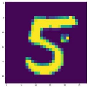  Fig.1: Example of a trigger and its location Basic Definitions and Notations: $N$ —neural network; $I$ — an image that is analyzed in terms of the presence of a trigger; $X$ — set of images $I$, which is checked by the algorithm; $n$ — number of pixels in the image; $x_{i}$ — the value of the neuron before the one that is currently being analyzed; $x_{j}$ — calculated current value of the neuron; $x_{i}\in [l_{i},u_{i}]$ — range of values for each neuron; $$ \phi_ {p r e} = \left[ h _ {p}, w _ {p} \right] \leq j \leq \left[ h _ {p} + h _ {s}, w _ {p} + w _ {s} \right] \wedge 0 \leq x [ j ] \leq $$ 1— preconditions for pixels that may contain trigger; $(c_{s},h_{s},w_{s})$ — trigger parameters: number of channels, height and width, respectively; $(h_p, w_p)$ — upper left coordinate of the trigger; $t_s$ — output value of the neural network for the image with a trigger superimposed on it; $\theta$ — specified success probability value; $K$ — the number of images in the sample checked for the absence of a trigger, or the number of elements in the set $X$. A trigger is a rectangular sticker on an image that has the same number of channels and changes the classification (it is assumed that the trigger is the same for all images of a certain set and is located in the same place), for example, $a3 \times 3$ square with pixels of different colors in Fig.1. Formal definition: for a neural network solving the problem of classifying images of size $(c, h, w)$, the trigger is some image $S$ of size $(c_s, h_s, w_s)$ such that $c_s = c, h_s \leq h, w_s \leq w$. We can say that in the picture $I$ there is a trigger of $\mathrm{size}(c_s, h_s, w_s)$, the upper left corner of which is located at the place $(h_p, w_p)$ (subject to the obvious conditions $h_p + h_s \leq h, w_p + w_s \leq w$ ), if $$ \begin{array}{l} S [ c _ {i}, h _ {i} - h _ {p}, w _ {i} - w _ {p} ], j f \\I _ {[ c, b, w ]} = \int \left(h _ {p} \leq h _ {i} < h _ {p} + h _ {s}\right) \wedge \\I _ {s} \left[ c _ {i}, n _ {i}, w _ {i} \right] - \mathrm {t} \wedge \left(w _ {p} \leq w _ {i} < w _ {p} + w _ {s}\right); \\I [ c _ {i}, h _ {i}, w _ {i} ], o t h e r w i s e. \\\end{array} $$ In other words, the trigger changes certain pixels of the image to given ones. Formal Statement of the Problem There is no patch (trigger) $S$ such that when applied to a certain set of images $I \in X$, the neural network $N$ changes the output class to the target class $t_s$, on images $I_s$ with the trigger $S$: $$ \nexists S \left(c _ {s}, h _ {s}, w _ {s}\right): \forall I _ {s} \in X: N \left(I _ {s}\right) = t _ {s}. $$ Initial conditions: 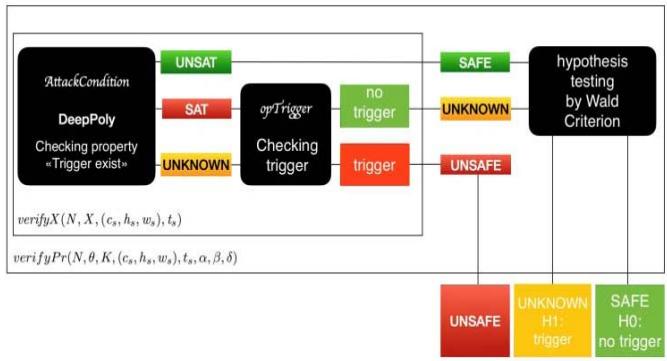 Fig. 3: Pseudocode for the verify Prfunction [1] Fig. 2: Flowchart of the algorithm for searching for a trigger 1. Dataset: MNIST — 10,000 images in $1 \times 28 \times 28$ format; neural networks: fully connected and convolutional with activation functions ReLU, Sigmoid, Tanh with the number of parameters up to 100,000; 2. Trigger Parameters: $1 \times 3 \times 3$, any pixel values in the area; 3. Security Property: no trigger; 4. Verification Algorithm: DeepPoly. ## II. ALGORITHM FOR SEARCHING FOR A TRIGGER IN AN IMAGE The algorithm [1] is based on the DeepPoly verifier [3]. Its main goal is to search for a trigger that consistently fools the classifier for a certain number of images. The output value of the artificial neural network changes to a predetermined value. The search is performed over the entire image and for all possible values of each trigger pixel (a $3 \times 3$ trigger is considered and tested, although other values are possible). The Wald Criterion [4] is also used to evaluate hypotheses about the occurrence of a trigger. Step by step, the entire algorithm works as follows: 1. Fix the position of the trigger. In the future, it is in this fixed area that there will be checking for the presence of a trigger; 2. We go through the set of images and build variations of images: a) Calculate for an artificial neural network and a given image a set of constraints. Constraints are calculated in the body of the attack Condition function; b) We pass these restrictions to the SAT solver, and look at the answer: if the formula is degenerate, then there is no trigger for the image, therefore, the neural network is resistant to triggers; ### c) Otherwise we add these restrictions to the previous ones; 3. If the SAT solver finds a counterexample, then, consequently, there is a trigger. We find it by gradually parsing the solution to a Boolean function, which is performed in the opTrigger function; 4. If the SAT solver confirmed that the set of constraints does not have a solution, then the neural network works correctly; 5. If the SAT solver could not confirm the degeneracy of the constraints, and a trigger was not found, then more research needs to be done. The relationships between the Attack Condition, opTrigger functions and all of the listed methods are presented in the block diagram in Fig. 2. a) Description of how the Verify Pr Function Works - The algorithm is represented by the function verify $\operatorname{Pr}$, which takes as input data the neural network $N$, the number of pictures $K$ in the sample being tested, all trigger indicators $(c_s, h_s, w_s)$, $t_s$ probabilistic parameters $\alpha, \beta, \delta$ of Wald criterion (SPRT) [4] and provides information about the presence or absence of a trigger with a given probability (Fig. 3). {"algorithm_caption":[{"type":"text","content":"Algorithm 1: verifyPr(N,θ,K,(cs,hsw),ts,α,β,δ) "}],"algorithm_content":[{"type":"text","content":"1 let "},{"type":"equation_inline","content":"n\\gets 0"},{"type":"text","content":" be the number of times verify "},{"type":"equation_inline","content":"X"},{"type":"text","content":" is called; \n2 let "},{"type":"equation_inline","content":"z\\gets 0"},{"type":"text","content":" be the number of times verify "},{"type":"equation_inline","content":"X"},{"type":"text","content":" returns SAFE; \n3 let "},{"type":"equation_inline","content":"p_0\\gets (1 - \\theta^K) + \\delta,p_1\\gets (1 - \\theta^k) - \\delta;"},{"type":"text","content":" \n4 while true do \n5 "},{"type":"equation_inline","content":"n\\gets n + 1;"},{"type":"text","content":" \n6 randomly select a set of images "},{"type":"equation_inline","content":"X"},{"type":"text","content":" with size "},{"type":"equation_inline","content":"K"},{"type":"text","content":". \n7 if verify "},{"type":"equation_inline","content":"X(N,X,(c_s,h_s,w_s),t_s)"},{"type":"text","content":" returns SAFE then \n8 "},{"type":"equation_inline","content":"\\begin{array}{r}\\lfloor z\\leftarrow z + 1; \\end{array}"},{"type":"text","content":" \n9 else if verify "},{"type":"equation_inline","content":"X(N,X,(c_s,h_s,w_s),t_s)"},{"type":"text","content":" returns UNSAFE then \n10 if the generated trigger satisfies the success rate then \n11 return UNSAFE; \n12 if "},{"type":"equation_inline","content":"\\frac{p_1^z}{p_0^z}\\times \\frac{(1 - p_1)^{n - z}}{(1 - p_0)^{n - z}}\\leq \\frac{\\beta}{1 - \\alpha}"},{"type":"text","content":" then \n13 return SAFE; // Accept "},{"type":"equation_inline","content":"H_{0}"},{"type":"text","content":" \n14 else if "},{"type":"equation_inline","content":"\\frac{p_1^z}{p_0^z}\\times \\frac{(1 - p_1)^{n - z}}{(1 - p_0)^{n - z}}\\geq \\frac{1 - \\beta}{\\alpha}"},{"type":"text","content":" then \n15 return UNKNOWN; // Accept "},{"type":"equation_inline","content":"H_{1}"}]} [lines 1-2] Two variables are introduced: $n$ — the number of calls to the verify X function, $z$ — the number of SAFE responses returned by the verify X function. [line 3] Set the probabilities $p_0, p_1$ for using SPRT. [line 4] A loop is started that runs until the SPRT conditions are met, as soon as the test monitors the fulfillment of one of the conditions, the result is given which hypothesis should be accepted [lines 12-15]. [line 5] A counter is started for the number of calls to the verify X function. [line 6] Selecting $K$ images randomly and composing them into a verifiable set $X$, which is fed to the input of the verifyX function. [lines 7-11] Application of the verifyX function, which will be described in the following pseudocode (Fig. 4). The SAFE output means that you need to increase the $z$ variable by 1 and go to a new iteration of SPRT, the UNSAFE output checks that the flip-flop does not satisfy all the specified statistical parameters and moves on to SPRT. ### b) Description of how the Verify X Function Works The verify $X$ function takes as input the neural network $N$, the tested set of images $X$, the dimensions $(c_s, h_s, w_s)$ and position $(h_p, w_p)$ of the trigger, the target label for the trigger $t_s$. {"algorithm_caption":[{"type":"text","content":"Algorithm 2: verify "},{"type":"equation_inline","content":"X(N, X, (c_s, h_s, w_s), t_s)"}],"algorithm_content":[{"type":"text","content":"1 let hasUnknown "},{"type":"equation_inline","content":"\\leftarrow"},{"type":"text","content":" false; \n2 foreach trigger position "},{"type":"equation_inline","content":"(h_p,w_p)"},{"type":"text","content":" do \n3 let "},{"type":"equation_inline","content":"\\phi \\gets \\phi_{pre}"},{"type":"text","content":". \n4 foreach image "},{"type":"equation_inline","content":"I\\in X"},{"type":"text","content":" do \n5 let "},{"type":"equation_inline","content":"\\phi_I\\gets"},{"type":"text","content":" attackCondition(N,I, "},{"type":"equation_inline","content":"\\phi_{pre},(c_s,h_s,w_s),(h_p,w_p),t_s)"},{"type":"text","content":". \n6 if "},{"type":"equation_inline","content":"\\phi_I"},{"type":"text","content":" is UNSAT then \n7 "},{"type":"equation_inline","content":"\\begin{array}{r}\\phi \\gets \\mathrm{false};\\\\ \\mathrm{break}; \\end{array}"},{"type":"text","content":" \n8 else \n9 else \n10 "},{"type":"equation_inline","content":"\\begin{array}{rl} & {\\phi \\gets \\phi \\wedge \\phi_I;}\\\\ & {\\phi \\gets \\phi \\wedge \\phi_I;} \\end{array}"},{"type":"text","content":" \n11 if solving "},{"type":"equation_inline","content":"\\phi"},{"type":"text","content":" results in SAT or UNKNOWN then \n12 if opTrigger(N,X, "},{"type":"equation_inline","content":"\\phi,(c_s,h_s,w_s),(h_p,w_p),t_s)"},{"type":"text","content":" returns a trigger then \n13 return UNSAFE; \n14 else \n15 hasUnknown "},{"type":"equation_inline","content":"\\leftarrow"},{"type":"text","content":" true; \nreturn hasUnknown?UNKNOWN:SAFE; "}]} Fig. 4: Pseudo code for the verify X function [1] At the output, the verify $X$ function produces the response SAFE if there is no trigger in the selected set $X$ or UNSAFE if there is a trigger (Fig. 2). [line 1] The has Unknown variable is created, which is responsible for the case of uncertainty (it is impossible to get an answer about the presence or absence of a trigger), by default its value is set to False. [line 2] The cycle is started to cycle through all possible trigger locations on the image being checked. [line 3] The neural network is specified by a set of conjunctions $\phi$, that is, in a form accessible to the SAT solver. During initialization, a set of initial constraints $\phi_{pre} = \Lambda_{j \in P(w_p, h_p)} l w_j \leq x_j \leq u p_j$ for the value of pixels $x_j$ located at positions $j \in P(w_p, h_p)$ in which the location is assumed at this step is entered into this variable trigger. Herelw and up are normalized boundaries for the trigger value, lying in the interval [0; 1]. [line 4] For each image $I \in X$, a cycle is started to check each image for the presence of a trigger. [line 5] The main function for checking the presence of a trigger attack Condition uses the DeepPoly formal verification algorithm for neural networks, which checks the property "there is a trigger on the image", returns an image represented in the form of conjunctions $\phi_I$, and a SAT response if the property is satisfied (trigger found), UNSAT - property not satisfied (trigger not found). [lines 6-10] If the attack Condition function returned UNSAT in the previous step, then the neural network is not executable, the variable $\phi$ is assigned the value False, exiting the loop. If a trigger is found, then its representation $\phi_{I}$ is added to the neural network function. [lines 11-15] The resulting representation of the neural network $\phi$ is fed into the SAT solver, and if the output is SAT or UNKNOWN, then the opTrigger function is run. ## i. The function opTigger First checks whether the resulting rectangle $S$ of size $(c_s, h_s, w_s)$ at position $(h_p, w_p)$ is a trigger that successfully attacks every image $I$ in the test set $X$. Because If the accumulated error of abstract interpretation resulting from the application of the DeepPoly algorithm is too large, the resulting model may be a false trigger. If it is a real trigger, then it returns model $S$ and the output is UNSAFE. The opTrigger function creates a trigger based on the available data, using an approach based on optimizing the loss function: $$ l o s s (N, I, S, (h _ {p}, w _ {p}), t _ {s}) = \left\{ \begin{array}{c l} 0, & \text{if } n _ {s} > n _ {0}; \\ n _ {0} - n _ {s} - \epsilon, & \text{otherwise.} \end{array} \right. $$ $n_{s} = N(I_{s})[t_{s}]$ — outputfor target label $t_{s}$; $n_{0} = \max_{j \neq t_{s}} N(I_{s})[j]$ — next after the largest value of the output vector; $\epsilon$ is a small constant, about $10^{-9}$. The loss function returns 0 if the attack on $I$ by the trigger is successful. Otherwise, it returns a quantitative measure of how far the simulated attack is from being successful. For the entire tested set $X$ we obtain a joint loss function $$ \operatorname{loss} (N, X, S, \left(h _ {p}, w _ {p}\right), t _ {s}) = \sum_ {I \in X} \operatorname{loss} (N, I, S, \left(h _ {p}, w _ {p}\right), t _ {s}) $$ An optimization problem is then solved to find an attack that successfully changes the classification of all images in $X$: $\text{argmin}_S \text{loss}(N, X, S, (h_p, w_p), t_s)$. ## ii. The Attack Condition Function Takes all parameters as input and outputs the result 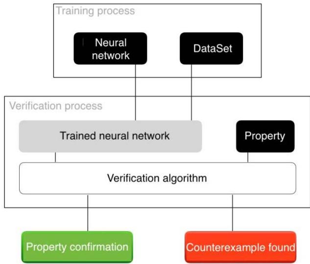 Fig. 7: Pseudo code for the Deep Poly ReLU function Fig. 5: Pseudocode for the Attack Condition function there is a trigger or not a trigger (Fig. 5). Inserts restrictions on the trigger in the form of conjunctions and adds $\phi$ to the network structure. The main idea of checking for a trigger: the area of pixels in which the trigger will be placed is selected, each such pixel is assigned a symbolic value included in the interval [0; 1] [lines 1-8]. Next, using the DeepPolyReLU function, we track the moment at which the checked pixel value from the segment [0; 1] will change the output vector of values, that is, the classification will change, we obtain the pixel value at which the trigger will be located on this pixel [lines 9-21]. If for all values of the checked pixel from the segment [0; 1] there is no change in the value of the target label (the output segment for the target label at all points is greater than the output segments for all other values) [line 25], then there will be no trigger, we return UNSAT [line 26], if it is not clear whether the target label has changed or not (the output segment for the target label intersects with some output segment for some of the other values), then the situation requires moredeep analysis, UNKNOWN is returned [lines 29 and 37]. If the output label has definitely changed, then the trigger is found, SAT is returned [line 35]. The DeepPoly algorithm [3], like formal verification algorithms [5], checks properties (Fig. 6). In the context of the verifyX function, the "no trigger" property is checked. {"algorithm_caption":[],"algorithm_content":[{"type":"text","content":"Algorithm 1 attackCondition "},{"type":"equation_inline","content":"(N,I,(c_s,h_s,w_s),(h_p,w_p),t_s)"},{"type":"text","content":" \n1: let constraints "},{"type":"equation_inline","content":"\\leftarrow [[0,0]]\\ast (h\\ast w)"},{"type":"text","content":" \n2: for "},{"type":"equation_inline","content":"j\\gets 0,\\dots,h\\ast w"},{"type":"text","content":" do \n3: if "},{"type":"equation_inline","content":"j\\in \\phi_{pre}"},{"type":"text","content":" then \n4: constraints "},{"type":"equation_inline","content":"[j]\\gets ([0,1])"},{"type":"text","content":" \n5: else \n6: constraints "},{"type":"equation_inline","content":"[j]\\gets ([I[j],I[j]])"},{"type":"text","content":" \n7: end if \n8: end for \n9: foreach layer "},{"type":"equation_inline","content":"\\in N"},{"type":"text","content":" do \n10: if layer is ReLU then \n11: for "},{"type":"equation_inline","content":"i\\gets 0,\\ldots,len(\\mathrm{constraints})"},{"type":"text","content":" do \n12: constraints[i] "},{"type":"equation_inline","content":"\\leftarrow"},{"type":"text","content":" DeepPolyReLU(constraints[i][0],constraints[i][1]); \n13: end for \n14: else \n15: NewConstraints "},{"type":"equation_inline","content":"\\leftarrow [[0,0]]\\ast ("},{"type":"text","content":" layer.CountNeurons); \n16: for "},{"type":"equation_inline","content":"i\\gets 0\\dots \\mathrm{len}(\\mathrm{layer}.Count\\mathrm{Neurons})"},{"type":"text","content":" do \n17: NewConstraints[i] "},{"type":"equation_inline","content":"\\leftarrow"},{"type":"text","content":" AffineCompute(constraints, layerweights[i], layer.bias[s]); \n18: constraints "},{"type":"equation_inline","content":"\\leftarrow"},{"type":"text","content":" NewConstraints; \n19: end for \n20: end if \n21: end for \n22: let flag "},{"type":"equation_inline","content":"\\leftarrow"},{"type":"text","content":" True \n23: for "},{"type":"equation_inline","content":"i\\gets 0,\\ldots,len(\\mathrm{constraints})"},{"type":"text","content":" do \n24: if "},{"type":"equation_inline","content":"i\\neq t_s"},{"type":"text","content":" then \n25: if constraints[t_s][1] < constraints[i][0] then return UNSAT; \n27: else \n28: if constraints[t_s][0] < constraints[i][1] then flag "},{"type":"equation_inline","content":"\\leftarrow"},{"type":"text","content":" False; \n30: end if \n31: end if \n32: end if \n33: end for \n34: if flag then \n35: return SAT; \n36: else \n37: return UNKNOWN; \n38: end if "}]} Fig. 6: General scheme of operation of algorithms for formal verification of neural networks ### c) Deep Poly ReLU function Analyzes approximate values for the output of the ReLU activation function (Fig. 7). {"algorithm_caption":[],"algorithm_content":[{"type":"text","content":"Algorithm 2 DeepPolyReLU(l,u) \n1: if "},{"type":"equation_inline","content":"0\\in [l_i,u_i]"},{"type":"text","content":" then \n2: let "},{"type":"equation_inline","content":"S_{1}\\gets (u_{i} - l_{i})*u_{i} / 2"},{"type":"text","content":" \n3: let "},{"type":"equation_inline","content":"S_{2}\\leftarrow (u_{i} - l_{i})*(-l_{i}) / 2"},{"type":"text","content":" \n4: if "},{"type":"equation_inline","content":"S_{1} < S_{2}"},{"type":"text","content":" then \n5: return "},{"type":"equation_inline","content":"[0,u_i]"},{"type":"text","content":" \n6: else \n7: return "},{"type":"equation_inline","content":"[l_i,u_i]"},{"type":"text","content":" \n8: end if \n9: else \n10: if "},{"type":"equation_inline","content":"u_{i} < 0"},{"type":"text","content":" then \n11: return "},{"type":"equation_inline","content":"[0,0]"},{"type":"text","content":" \n12: else \n13: return "},{"type":"equation_inline","content":"[l_i,u_i]"},{"type":"text","content":" \n14: end if \n15: end if "}]} ### d) Basic Moments - Linear constraints on each neuron are represented as a linear combination of only input data $x_{1}, x_{2}$ (and not through the constraints of previous neurons), then the constraints for each neuron at each step will be better, the segment will expand less. - If the ReLU input receives a segment with a halfliving ends, then it turns into itself, without changes. If the segment contains a point zero, then as constraints we use $0 \leq x_{j} \leq \lambda x_{i} + \mu$ (the equation of the straight line defining the upper boundary of the triangle passing through the points $(l_i;0)$, $(u_i;u_i)$, $l_i$ and $u_i$ — boundaries of the interval in the previous step). If the entire segment is negative, then it simply goes to zero. - The main difference from other algorithms is exactly one lower constraint. This makes it possible to narrow the boundaries of the intervals and facilitate computing power (Fig. 8). It is also argued that approximation by such triangles is better than zonotopes — they are easier to calculate, and also often have a smaller area. With a similar formulation of the problem, the zonotope in this case will be a parallelogram, the lower side of which contains the point $(0;0)$.   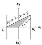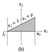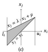 Fig.10: Errors of type 1 and 2 Fig. 8: Approximation of the ReLU function in the DeepPoly algorithm [3] The AttackCondition function takes all parameters as input and outputs the result — there is a trigger or there is no trigger. Inserts restrictions on the trigger in the form of conjunctions and adds $\phi$ to the network structure. These results are then used in the VerifyPr function, which gives a probabilistic assessment of the presence of a trigger. ### e) The Affine Compute Function Takes as input values from the previous layer, performs standard affine transformations — multiplying by weights and adding a bias vector, and at the output produces an interval within which all possible values supplied to the input of the ReLU function lie (Fig. 9). {"algorithm_caption":[],"algorithm_content":[{"type":"text","content":"Algorithm 3 AffineCompute(constraints, w, bias) \n1: let "},{"type":"equation_inline","content":"l_j \\gets \\text{bias}"},{"type":"text","content":"; \n2: let "},{"type":"equation_inline","content":"u_j \\gets \\text{bias}"},{"type":"text","content":"; \n3: for "},{"type":"equation_inline","content":"i \\gets 0, \\dots, \\text{len}(\\text{constraints})"},{"type":"text","content":" do \n4: "},{"type":"equation_inline","content":"l_j \\gets l_j + w[i] * \\text{constraints}[i][0]"},{"type":"text","content":"; \n5: "},{"type":"equation_inline","content":"u_j \\gets u_j + w[i] * \\text{constraints}[i][1]"},{"type":"text","content":"; \n6: end for \n7: return "},{"type":"equation_inline","content":"[l_j, u_j]"},{"type":"text","content":"; "}]} Fig. 9: Pseudocode for the AffineCompute function ### f) SPRT (Sequential Probability Ratio Test) or Wald Criterion Designations: $\theta$ is the probability of a trigger appearing, common to all $K$ pictures: for a given neural network $N$, trigger $S$, target label $t_s$, it is postulated that $S$ has a probability of success $\theta$ if and only if there is a position $(h_p, w_p)$ such that the probability of occurrence $L(N(I_s)) = \arg\max_i(y_{output}) = t_s$ for any $I$ in the chosen test set is $\theta$. No trigger: $$ \forall I \in X \exists s, I _ {s} = I (s): L \left(N \left(I _ {s}\right)\right) > t _ {s}, $$ where $\alpha, \beta, \delta$ are confidence levels. Testable hypotheses: $H_{0}$: The probability of no attack on a set of Krandomlyselected images is greater than $1 - \theta^{K}$. $H_{1}$: The probability of no attack on a set $K$ of randomly selected images is no greater than $1 - \theta^{K}$. Next, the researcher sets the values of the parameters $\alpha$ and $\beta$, this is the probability of an error of the first and second kind, respectively (Fig. 10). Decision <table><tr><td>Truth</td><td>accept H0, reject H1</td><td>reject H0, accept H1</td></tr><tr><td>p ≥ θ: H0 true, H1 false</td><td>correct (&gt;1 - α)</td><td>type I error (≤α)</td></tr><tr><td>p &lt; θ: H0 false, H1 true</td><td>type II error (≤β)</td><td>correct (&gt;1 - β)</td></tr></table> Parameter $\delta$ is the "gap" between the null and alternative hypothesis. If the value falls in a region where the estimated probability of not having the attack will be greater than $p_0 = (1 - \theta^K) + \delta$, then we accept the null hypothesis, if less than $p_1 = (1 - \theta^K) - \delta$, then we reject the null hypothesis, if between them, then we move on to a new iteration of the algorithm. This is precisely the procedure of sequential analysis, which consists in sequential testing of the indicated inequalities for probabilities, and in this way it differs from simple testing of hypotheses. The article [1] sets the following parameter values $K = 5,10,100,\theta = 0.8,0.9,1,\alpha = \beta = \delta = 0.01$. ## III. EXPERIMENTAL PART ### a) Scalability Study A scalability study showed that for neural networks with about 10,000 parameters, searching for triggers for all 10 labels takes about several minutes. In article [1] and the implementation, a search for triggers for the conv_small_relu neural network was proposed (the architecture is shown in Fig. 11). Such a neural network contains 89,000 parameters. Finding triggers for all 10 tags takes about 10 hours. 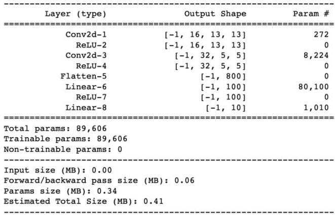 Fig. 11: Neural networkconv_small_relu architecture Similar architectures with fewer and more parameters were tested. For neural networks with about 105,000 parameters, verification for one target label takes about 20 hours (for 10 labels it takes approximately 200 hours). From this we conclude that the duration of verification increases exponentially with increasing number of parameters. ### b) Improved Work Speed During the analysis of the repository, the bottleneck was identified — the back_substitute function of the utils.py module, which is responsible for the integration of interval arithmetic. Profiling of this program shows that about $70\%$ of the execution time is occupied by this function (Fig. 12). The calculation graph shows similar results (Fig. 13).  Fig.12: Table of execution times of all algorithm functions To optimize the selected bottleneck, various approaches to code optimization and library replacement were tested, as well as deployment on GPUs using the PyTorch library.  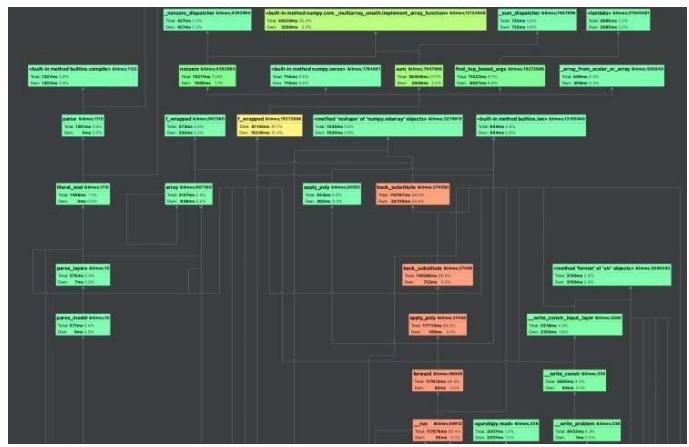Fig.13. Calculation graph of all algorithm functions It was not possible to obtain a significant increase in performance using the GPU, since the method uses a large number of not very complex calculations. As a result, calculations slowed down 10 times. This happened because GPUs are adapted for calculating large matrices, while the CPU copes better with the proposed task. The use of other libraries and code optimization led to a 20 percent improvement in the execution speed of the back_substitute function. The overall running time of the algorithm was also improved by approximately $10\%$ (Fig. 14). 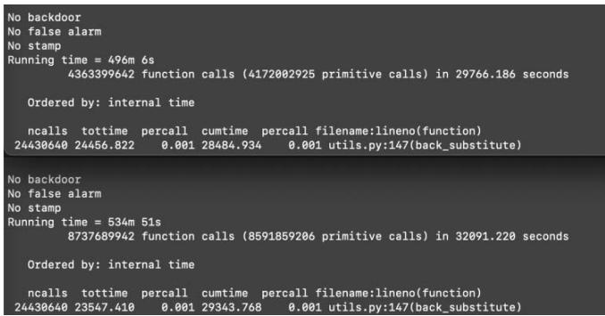 Fig.14: Comparison of algorithm running time before and after optimization improvements Parallelization of the selected problem is impossible, since the newly calculated data must again be fed into the input. Nevertheless, you can try to parallelize the search for a trigger in different places, but this issue is subject to deeper study. ## IV. PRACTICAL IMPLEMENTATION ### a) Software and Hardware The main part of the described experiments was carried out on a computer complex using a central processor and having the following characteristics: Table I: Hardware <table><tr><td>CPU</td><td>Apple M1 Max processor</td></tr><tr><td>RAM</td><td>32 GB</td></tr></table> Experiments on the GPU were carried out using a computing cluster with the characteristics indicated in Table II. Table II: Hardware, GPU cluster <table><tr><td>Video card</td><td>NVIDIA RTX A6000</td></tr><tr><td>Processor</td><td>AMD EPYC 7532 32-Core</td></tr><tr><td>RAM</td><td>252 GB</td></tr></table> Software with the characteristics shown in Table III was used. Table III: Software <table><tr><td>OS (CPU)</td><td>MacOS Ventura 13.3.1</td></tr><tr><td>OS (GPU)</td><td>Ubuntu 20.04.4 LTS</td></tr><tr><td>Python</td><td>3.10.0</td></tr><tr><td>numpy</td><td>1.23.5</td></tr><tr><td>scipy</td><td>1.8.0</td></tr><tr><td>autograd</td><td>1.4</td></tr><tr><td></td><td>9.5.1</td></tr><tr><td>torchsummary</td><td>1.5.1</td></tr><tr><td>nvidia CUDA</td><td>11.7</td></tr><tr><td>pytorch</td><td>1.13.1</td></tr></table> ### b) Datasets and Neural Networks Neural networks trained on the following data sets were used: - MNIST - a set of single-channel images of $28 \times 28$ pixels. Images are divided into 10 classes — numbers from 0 to 9 (Fig. 15); - CIFAR-10 - a set of three-channel images of $32 \times 32$ pixels. Images are divided into 10 classes — airplane, car, bird, cat, deer, dog, frog, horse, ship, truck (Fig. 16). In addition to the experiments proposed in the article, other neural networks were trained. They were analyzed using a trigger search algorithm and used to compare the original implementation and the optimized version. Neural networks that showed high accuracy on the test set, as a rule, did not have a trigger. An example of a tested neural network is shown in Fig. 11.  Fig.15: MNIST DataSet 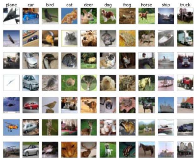 Fig.16: CIFAR-10 DataSet ### c) Disadvantages of the Current Implementation Formal verification, as a young field of science, has many difficulties with uniform standards of use. The proposed implementation of the trigger search problem has a number of significant problems that arise for the user who decides to use this algorithm. It was decided to correct the identified deficiencies as part of this work. 1. The proposed implementation works only with neural networks stored in a special format, where all weights and biases are stored in separate txt files, and the architecture itself is written in a separate spec.json file. To read neural networks in this format, a separate json_parser module is used, which extracts the weights of the neural network and prepares them for work. The inability to conduct an experiment on a neural network not described by the authors is a significant drawback; 2. The proposed algorithm works quite slowly even on small neural networks, which is natural, since formal verification very carefully analyzes the entire neural network layer by layer, neuron by neuron. Since when testing more complex neural networks with a large number of parameters, the key limitation is the running time of the algorithm, optimizing it will increase its applicability. Also, the existing implementation does not use parallelization and it was decided to fix this too; 3. The existing implementation is only suitable for testing neural networks trained on the MNIST 3. To support the CIFAR-10 data set, the images in it were normalized from 0 to 1 and converted into the appropriate specialized format. The existing implementation was adapted to use a $3 \times 3 \times 3$ trigger, and support for multi-channel triggers was added wherever this was lacking. Table V: Algorithm running time before and after optimization <table><tr><td>Neural network</td><td>Number of parameters</td><td>Original time</td><td>Optimized time</td></tr><tr><td>mnist_model_0</td><td>79 510</td><td>1 223 s</td><td>341 s</td></tr><tr><td>mnist_model_1</td><td>159 010</td><td>2 352 s</td><td>659 s</td></tr><tr><td>mnist_model_2</td><td>199 310</td><td>6 873 s</td><td>1 704 s</td></tr><tr><td>mnist_model_3</td><td>119 810</td><td>5 394 s</td><td>1 328 s</td></tr><tr><td>mnist_conv_small</td><td>89 606</td><td>22 452 s</td><td>4 548 s</td></tr><tr><td>mnist_model_5</td><td>159 387</td><td>258 854 s</td><td>74 855 s</td></tr><tr><td>mnist_conv_maxpool</td><td>34 622</td><td>17 880 s</td><td>3 632 s</td></tr><tr><td>cifar_conv_relu</td><td>62 006</td><td>—</td><td>197 426 s</td></tr></table> ### f) Assessing the complexity of the trigger search algorithm in neural networks of various architectures The time it takes to search for a trigger in a neural network depends on its architecture. The complexity of testing a neural network can be determined both empirically and theoretically. It will correlate with the number of parameters and depend on: the number of layers in the neural network, the size of these layers, the type of these layers. Empirically, it was found that fully connected layers are faster to check than convolutional layers. The verification time depends to a greater extent on the number of layers and to a lesser extent on their size. The number of parameters for verifying fully connected layers can be expressed as $O(m * n)$, where $m$ and $n$ are the number of inputs and outputs of the layer. The number of parameters for verifying 2D layers can be expressed as $O(c * h * w)$ for Conv2D and $O(c * h^2 * w^2)$ for MaxPool2D, where $c, h$ and $w$ are the number of channels, the height and width of the kernel. Thus, it is easy to see that the more parameters the 2D layers have, the longer the neural network will take to verify. Table VI: Estimation of the complexity of searching for a trigger for different types of layers <table><tr><td>Layer type</td><td>Complexity</td></tr><tr><td>Linear</td><td>O(m*n)</td></tr><tr><td>Conv2D</td><td>O(c*h*w)</td></tr><tr><td>MaxPool2D</td><td>O(c*h2*w2)</td></tr></table> ## V. CONCLUSION Formal verification algorithms are generally applicable to checking neural networks for the absence of attacks. Using the DeepPoly algorithm, you can not only check for the presence of a trigger in an image, but also generate triggers. Verification problems arise on networks containing Sigmoid and Tanh activation functions. Probabilistic models provide a numerical assessment of testing the operation of neural networks; they can be combined with formal verification algorithms. As a continuation of the work, you can try to use other verification algorithms for these experiments, based on the analysis by zonotopes [5] of the Sigmoid and Tanh activation functions.

Generating HTML Viewer...

References

7 Cites in Article
Pham Long,H,Sun Jun (2022). Verifying neural networks against backdoor attacks.
Deng Li (2012). The mnist database of handwritten digit images for machine learning research.
Gagandeep Singh,Timon Gehr,Markus Püschel,Martin Vechev (2018). Replication Package for the article.
Gagandeep Singh,Timon Gehr,Markus Püschel,Martin Vechev (2019). An abstract domain for certifying neural networks.
Wald (1945). Sequential tests of statistical hypotheses.
Ekaterina Stroeva,Aleksey Tonkikh (2022). Methods for formal verification of artificial neural networks: A review of existing approaches//Interna-tional Journal of Open Information Technologies.
V CONCLUSION Optimizing the Running Time of a Trigger Search Algorithm based on the Principles of Formal Verification of Artificial Neural Networks.
No ethics committee approval was required for this article type.
Data Availability
Not applicable for this article.
How to Cite This Article
Aleksey Tonkikh. 2026. \u201cOptimizing the Running Time of a Trigger Search Algorithm Based on the Principles of Formal Verification of Artificial Neural Networks\u201d. Global Journal of Computer Science and Technology - D: Neural & AI GJCST-D Volume 24 (GJCST Volume 24 Issue D1).
Explore published articles in an immersive Augmented Reality environment. Our platform converts research papers into interactive 3D books, allowing readers to view and interact with content using AR and VR compatible devices.
Your published article is automatically converted into a realistic 3D book. Flip through pages and read research papers in a more engaging and interactive format.
Our website is actively being updated, and changes may occur frequently. Please clear your browser cache if needed. For feedback or error reporting, please email [email protected]
Thank you for connecting with us. We will respond to you shortly.