## I. INTRODUCTION It is well known that linear theory of elasticity describes the effective properties of various materials like steel, wood and concrete etc. But this theory is unable to explore the nano mechanical applications like nano structure vibrations, nano device stability etc. The theory of nonlocal elasticity is of great importance in determining the properties of nano structure and wave propagation. The nonlocal theory of elasticity takes account of remote action between atoms because in nonlocal elasticity, stresses at a point not only depend on strain at that point but also on all points of the body. Eringen[1-3]elaborated the concept of nonlocality to elasticity and proposed the theory of nonlocal elasticity. Eringen and Edelen[4] obtained constitutive equations for the nonlinear theory. Gurtin[5] gave linear thermoelastic model to investigate the stresses produced to temperature field and distribution of temperature due to action of internal forces. Nowacki[6-7] constructed asymptotic solution of boundary value problems of three dimensional micropolar theory of elasticity with free field of rotations and displacements. Green and Naghdi[8-9] introduced a new thermodynamical theory which uses a general entropy balance and discussed thermoelastic behaviour without energy dissipation. Kupradze et.al.[10] discussed three dimensional problem of the mathematical theory of elasticity and thermoelasticity. Kumar and Kumar[11] studied plane wave propagation in nonlocal micropolar thermoelastic material with voids. Kaur and Singh[12] studied propagation of plane wave in a nonlocal magneto-thermoelastic semiconductor solid with rotation and identified four types of reflected coupled longitudinal waves. Diffusion is the spontaneous movement of anything generally from a region of higher concentration to that of lower concentration and thermal diffusion makes use of heat transfer. The thermoelastic diffusion in elastic solids is due to coupling of mass diffusion field of temperature and that of strain in addition to mass and heat exchange with environment. Auoadi[13-16] derived equation of motion and constitutive equations for a generalized thermoelastic diffusion with one relaxation time and obtained variation principle for the governing equations. He proved uniqueness theorem for these equations by using Laplace transform. Free vibration of a thermoelastic diffusive cylinder was investigated by Sharma et al.[17]. Hörmander[18-19] contained analysed the partial differential operators which are very useful in order to find fundamental solution in the thermoelastic diffusion solid. To examine boundary value problem of thermoelasticity, it is mandatory to evaluate the fundamental solution of the system of partial differential equation and to discuss their basic properties. Fudamental solution in the classical theory of coupled thermoelasticity was firstly studied by Hetnarski[20-21]. Svanadze[22-25] obtained fundamental solution of equations of steady oscillations in different types of thermoelastic solids. Scarpetta[26], Ciarletta et al.[27], Svanadze et al.[28] found fundamental solution in the theory of micropolar elasticity. Fundamental solution in the theory of thermoelastic diffusion is established by Kumar and Kansal[29-30]. Many problems related to plane wave propagation and fundamental solution have been studied by some of other researchers like Sharma and Kumar[31], Kumar[32], Kumar et.al.[33], Kumar and Devi[34], Biswas[35], Kumar and Batra[36], Biswas[37-38], Kumar et al.[39], Poonam et al.[40], Kumar and Batra[41]. However, from the best of author's knowledge, no study has been done for investigating the combining effect of nonlocal and diffusion on fundamental solution of homogenous isotropic thermoelastic solid. In current problem, we have discussed plane wave propagation and established the fundamental solution of differential equations in case of steady oscillations in terms of elementary functions for nonlocal homogenous isotropic thermoelastic solid with diffusion. Some basic properties and special case are also discussed. ## II. BASIC EQUATIONS In three-dimensional Euclidean space $E^3$, let $\mathbf{X} = (x, y, z)$ be a point, $t$ represents the time variable and $\mathbf{D}_x \equiv (\frac{\partial}{\partial x}, \frac{\partial}{\partial y}, \frac{\partial}{\partial z})$. Following Eringen [1-3], the constitutive relations for nonlocal generalised thermoelastic solid with diffusion are given by $$ \left(1 - \varepsilon^ {2} \nabla^ {2}\right) \sigma_ {i j} = \sigma_ {i j} ^ {\prime} = 2 \mu e _ {i j} + \left[ \lambda e _ {k k} - \beta_ {1} T - \beta_ {2} C \right] \delta_ {i j} \tag {1} $$ $$ e _ {i j} = \frac {1}{2} \left(u _ {i, j} + u _ {j, i}\right) \tag {2} $$ Using constitutive relations, equation of motion for nonlocal homogenous isotropic thermoelastic solid with diffusion is $$ \mu u _ {i, j j} + (\lambda + \mu) u _ {j, i j} - \beta_ {1} T _ {, i} - \beta_ {2} C _ {, i} = \rho (1 - \varepsilon^ {2} \nabla^ {2}) \ddot {u} _ {i} \tag {3} $$ Equations of heat conduction and mass diffusion for nonlocal homogenous isotropic thermoelastic solid with diffusion are given by $$ \rho C _ {E} (\dot {T} + \tau_ {0} \ddot {T}) + \beta_ {1} T _ {0} (\dot {e} _ {k k} + \tau_ {0} \ddot {e} _ {k k}) + a ^ {*} T _ {0} (\dot {C} + \tau_ {0} \ddot {C}) = K T _ {, i i} \tag {4} $$ $$ D^{*} \beta_2 e_{kk,ii} + D^{*} a^{*} T_{,ii} + (1 - \varepsilon^2 \nabla^2) (\dot{C} + \tau\ddot{C}) = D^{*} b^{*} C_{,ii} $$ where $\mathbf{u} = (u_{1}, u_{2}, u_{3})$ is the displacement vector; $\sigma_{ij}$ are the stress components and $e_{ij}$ are components of strain tensor; $e_{kk}$ is dilatation; $\sigma_{ij}'$ corresponds to the local thermoelastic solid with diffusion; $T$ is the temperature change measured from the absolute temperature $T_{0}$; $C_{E}$ denotes specific heat at constant strain; $K$ is the thermal conductivity; $\tau_{0}$ is the relaxation time parameter and $\tau$ is the relaxation time of diffusion; $C$ is the concentration; $D^{*}$ is the thermoelastic diffusion constant; $a^{*}$ and $b^{*}$ respectively measures the thermo-diffusion effects and diffusive effects; $\rho$ is mass density; $\beta_{1}, \beta_{2}$ are material coefficients with $\beta_{1} = (3\lambda + 2\mu)\alpha_{t}$, $\beta_{2} = (3\lambda + 2\mu)\alpha_{c}$, $\lambda$ and $\mu$ are Lame's constants; $\alpha_{t}$ the coefficient of linear thermal expansion and $\alpha_{c}$ is the coefficient of linear diffusion expansion; $\nabla^{2}$ denotes the Laplacian operator; $\varepsilon = e_{0}a$ is the nonlocal parameter; $e_{0}$ corresponds to the material constant; $a$ denotes the characteristic length; $\delta_{ij}$ is Kronecker delta. In the above equations, superposed dot represents the derivative with respect to time and ',' in the subscript denotes the partial derivatives with respect to $x, y, z$ for $i, j = 1,2,3$ respectively. For two-dimensional problem, we will suppose that all quantities related to the medium are functions of cartesian coordinates $x$, $z$ (i.e. $\frac{\partial}{\partial y} \equiv 0$ ) and time $t$ and are independent of $y$. Displacement vector is considered as $$ \mathbf {u} = \left(u _ {1}, 0, u _ {3}\right) \tag {6} $$ We define the following dimensionless quantities $$ x ^ {\prime} = \frac {\omega_ {1} x}{c _ {1}}, z ^ {\prime} = \frac {\omega_ {1} z}{c _ {1}}, u _ {1} ^ {\prime} = \frac {\rho \omega_ {1} c _ {1}}{\beta_ {1} T _ {0}} u _ {1}, u _ {3} ^ {\prime} = \frac {\rho \omega_ {1} c _ {1}}{\beta_ {1} T _ {0}} u _ {3}, $$ $$ t ^ {\prime} = \omega_ {1} t, T ^ {\prime} = \frac {T}{T _ {0}}, C ^ {\prime} = \frac {\beta_ {2}}{\beta_ {1} T _ {0}} C, \tau_ {0} ^ {\prime} = \omega_ {1} \tau_ {0}, \tau^ {\prime} = \omega_ {1} \tau \tag {7} $$ where $\omega_{1} = \frac{\rho C_{E}c_{1}^{2}}{K}$, $c_{1} = \sqrt{\frac{\lambda + 2\mu}{\rho}}$ Now using equation (7) in equations (3), (4), (5) and suppressing the primes, we obtain $$ \alpha_ {1} \nabla^ {2} \mathbf{u} + \alpha_ {2} \operatorname{grad} \operatorname{div} \mathbf{u} - \operatorname{grad} T - \operatorname{grad} C = \left(1 - \varepsilon_ {1} ^ {2} \nabla^ {2}\right) \ddot{\mathbf{u}} $$ $$ \tau_ {t} ^ {0} (\dot{T} + \alpha_ {3} div \dot{\mathbf{u}} + \alpha_ {4} \dot{C}) = \nabla^ {2} T $$ $$ \alpha_ {5} \nabla^ {2} d i v \mathbf{u} + \alpha_ {6} \nabla^ {2} T - \alpha_ {7} \nabla^ {2} C + (1 - \varepsilon_ {1} ^ {2} \nabla^ {2}) \tau_ {c} ^ {0} \dot{C} = 0 $$ where $$ \alpha_ {1} = \frac {\lambda + \mu}{\lambda + 2 \mu}, \alpha_ {2} = \frac {\mu}{\lambda + 2 \mu}, \alpha_ {3} = \frac {\beta_ {1} ^ {2} T _ {0}}{\rho K \omega_ {1}}, \alpha_ {4} = \frac {a ^ {*} \beta_ {1} T _ {0} c _ {1} ^ {2}}{K \omega_ {1} \beta_ {2}}, \alpha_ {5} = \frac {D ^ {*} \beta_ {2} ^ {2} \omega_ {1}}{\rho c _ {1} ^ {4}}, $$ $$ \alpha_ {6} = \frac {D ^ {*} a ^ {*} \omega_ {1} \beta_ {2}}{\beta_ {1} c _ {1} ^ {2}}, \alpha_ {7} = \frac {D ^ {*} b ^ {*} \omega_ {1}}{c _ {1} ^ {2}} \varepsilon_ {1} ^ {2} = \frac {\varepsilon^ {2} \omega_ {1} ^ {2}}{c _ {1} ^ {2}}, \tau_ {t} ^ {0} = 1 + \tau_ {0} \omega_ {1} \frac {\partial}{\partial t}, \tau_ {c} ^ {0} = 1 + \tau \omega_ {1} \frac {\partial}{\partial t} $$ The displacement vector $\mathbf{u}$ is related to the potential functions $\phi_1(x,z,t)$ and $\phi_{2}(x,z,t)$ as $$ u _ {1} = \frac {\partial \phi_ {1}}{\partial x} + \frac {\partial \phi_ {2}}{\partial z}, \quad u _ {3} = \frac {\partial \phi_ {1}}{\partial z} - \frac {\partial \phi_ {2}}{\partial x} \tag {11} $$ Using equation (11) in equations (8)-(10), we obtain $$ \left(\alpha_ {1} + \alpha_ {2}\right) \nabla^ {2} \phi_ {1} - T - C = \left(1 - \varepsilon_ {1} ^ {2} \nabla^ {2}\right) \ddot {\phi} _ {1} \tag {12} $$ $$ \alpha_ {1} \nabla^ {2} \phi_ {2} = \left(1 - \varepsilon_ {1} ^ {2} \nabla^ {2}\right) \ddot {\phi} _ {2} \tag {13} $$ $$ \left(\frac{\partial}{\partial t} + \tau_ {0} \omega_ {1} \frac{\partial^ {2}}{\partial t ^ { 2}}\right) \left(T + \alpha_ {4} C + \alpha_ {3} \nabla^ {2} \phi_ {1}\right) = \nabla^ {2} T $$ $$ \alpha_ {5} \nabla^ {4} \phi_ {1} + \alpha_ {6} \nabla^ {2} T - \alpha_ {7} \nabla^ {2} C + \left(1 - \varepsilon_ {1} ^ {2} \nabla^ {2}\right) \left(\frac{\partial}{\partial t} + \tau \omega_ {1} \frac{\partial^ {2}}{\partial t ^ {2}}\right) C = 0 $$ Equations (12), (14) and (15) show that $\phi_1, T$ and $C$ are coupled and $\phi_2$ remains decoupled. ## III. PLANE WAVE We consider a plane wave propagating in a nonlocal homogenous isotropic thermoelastic media with diffusion and assume the solution of the form $$ (\phi_ {1}, \phi_ {2}, T, C) = (\bar{\phi} _ {1}, \bar{\phi} _ { 2}, \bar{T}, \bar{C}) \exp \{i k (\mathbf{n}. \mathbf{r} - c t) \} $$ where $\omega = k c$ is the frequency, $c$ is the wave velocity, $k$ is the wave number, $\bar{\phi}_1$, $\bar{\phi}_2$, $\bar{T}$, $\bar{C}$ are undetermined amplitudes that depend on the time and coordinates $\mathbf{r} = (x,0,z)$, $\mathbf{n}$ is the unit vector. Using equation (16) in equations (12)-(15), we obtain $$ \left(B_{1}k^{2}+\omega^{2}\right)\bar{\phi}_{1}=\bar{T}+\bar{C} $$ $$ \left(B _ {2} k ^ {2} - \omega^ {2}\right) \bar {\phi} _ {2} = 0 \tag {18} $$ $$ \left(k ^ {2} - B _ {3}\right) \bar {T} - \alpha_ {4} B _ {3} \bar {C} + \alpha_ {3} B _ {3} k ^ {2} \bar {\phi} _ {1} = 0 \tag {19} $$ $$ \alpha_ {5} k ^ {4} \bar{\phi} _ {1} - \alpha_ {6} k ^ {2} \bar{T} + \left(B _ {4} k ^ {2} - B _ {5}\right) \bar{C} = 0 $$ where $$ B _ {1} = \varepsilon_ {1} ^ {2} \omega^ {2} - 1, B _ {2} = \alpha_ {1} - \varepsilon_ {1} ^ {2} \omega^ {2}, B _ {3} = i \omega + \tau_ {0} \omega_ {1} \omega^ {2} $$ $$ B _ {4} = \alpha_ {7} - \varepsilon_ {1} ^ {2} (i \omega) - \varepsilon_ {1} ^ {2} \tau \omega_ {1} \omega^ {2}, B _ {5} = i \omega + \tau \omega_ {1} \omega^ {2} $$ Solving equations (17), (19) and (20) for $\bar{\phi}_1$, $\bar{T}$, $\bar{C}$ we obtain a cubic equation in $k^2$ as $$ F _ {1} k ^ {6} + G _ {1} k ^ {4} + H _ {1} k ^ {2} + J _ {1} = 0 \tag {21} $$ where $$ F _ {1} = B _ {4} B _ {1} + \alpha_ {5}, J _ {1} = B _ {3} B _ {5} \omega^ {2} $$ $$ G _ {1} = \alpha_ {3} \alpha_ {6} B _ {3} + B _ {4} \omega^ {2} - B _ {1} B _ {3} B _ {4} + \alpha_ {3} B _ {3} B _ {4} - B _ {5} B _ {1} + \alpha_ {4} \alpha_ {5} B _ {3} - \alpha_ {4} \alpha_ {6} B _ {1} B _ {3} - \alpha_ {5} B _ {3} $$ $$ H _ {1} = - B _ {4} B _ {3} \omega^ {2} - B _ {5} \omega^ {2} + B _ {5} B _ {3} B _ {1} - \alpha _ {3} B _ {3} B _ {5} - \alpha _ {4} \alpha _ {6} B _ {3} \omega^ {2} $$ Solving equation (21), we obtain six values of $k$ in which three values $k_{1}, k_{2}, k_{3}$ correspond to positive $z$ -direction and the other three values of $k$ correspond to negative $z$ -direction. Corresponding to $k_{1}, k_{2}$ and $k_{3}$ there exist three coupled waves, namely, longitudinal wave(P), thermal wave(T) and mass diffusion wave(MD). The expressions for the phase velocity, attenuation coefficients, penetration depth and specific loss of above waves are evaluated as Phase Velocity: The phase velocities $v_{1}, v_{2}$ and $v_{3}$ of P-wave, T-wave, and MD-wave, respectively, are given by $$ v _ {j} = \frac {\omega}{\left| R e \left(k _ {j}\right) \right|} \quad j = 1, 2, 3 \tag {22} $$ Attenuation Coefficients: The attenuation coefficients $Q_{1}$, $Q_{2}$ and $Q_{3}$ of P-wave, T-wave and MD-wave, respectively, can be written as $$ Q _ {j} = I m \left(k _ {j}\right) \quad j = 1, 2, 3 \tag {23} $$ Penetration Depth: The penetration depth $D_{1}$, $D_{2}$ and $D_{3}$ of P-wave, T-wave and MD-wave, respectively, is defined as $$ D _ {j} = \frac {1}{\left| I m \left(k _ {j}\right) \right|} \quad j = 1, 2, 3 \tag {24} $$ Specific Loss: The Specific Loss $L_{1}$, $L_{2}$ and $L_{3}$ of P-wave, T-wave and MD-wave, respectively, are given by $$ L _ {j} = 4 \pi \left| \frac {\operatorname {R e} \left(k _ {j}\right)}{\operatorname {I m} \left(k _ {j}\right)} \right| \quad j = 1, 2, 3 \tag {25} $$ Solving equation(18), we obtain two values of $k$ in which one value $k_{4}$ corresponds to positive $z$ -direction representing transverse wave(SV) and other value of $k$ corresponds to negative $z$ -direction. The phase velocity of transverse wave is given by $v_{4} = \sqrt{B_{2}}$ ## IV. STEADY OSCILLATIONS Assume that displacement vector, temperature change and concentration are functions as $$ \left(\mathbf {u} (x, z, t), T (x, z, t), C (x, z, t)\right) = R e \left[ \left(\mathbf {u} ^ {*} (x, z, t), T ^ {*} (x, z, t), C ^ {*} (x, z, t)\right) e ^ {- i \omega t} \right] \tag {26} $$ Using equation (26) in equations (8),(9),(10), we obtain following system of equations of steady oscillations $$ \left[ \left(\alpha_ {1} - \omega^ {2} \varepsilon_ {1} ^ {2}\right) \nabla^ {2} + \omega^ {2} \right] \mathbf{u} * + \alpha_ {2} \operatorname{grad} \operatorname{div} \mathbf{u} * - \operatorname{grad} T * - \operatorname{grad} C * = 0 \tag{27} $$ $$ -\tau_{t}^{01} \left[ \alpha_{3} \operatorname{div} \mathbf{u}^{*} + \alpha_{4} C^{*} \right] + \left( \nabla^{2} - \tau_{t}^{01} \right) T^{*} = 0 $$ $$ \alpha_ {5} \nabla^ {2} div \mathbf{u} ^ {*} + \alpha_ {6} \nabla^ {2} T ^ {*} + \left[ \tau_ {c} ^ {0 1} - \left(\alpha_ {7} + \varepsilon_ {1} ^ {2} \tau_ {c} ^ {0 1}\right) \nabla^ {2} \right] C ^ {*} = 0 $$ $$ \tau_ {t} ^ {0 1} = - i \omega (1 - i \omega \tau_ {0}), \tau_ {c} ^ {0 1} = - i \omega (1 - i \omega \tau) $$ We define matrix differential operator $$ \mathbf {B} \left(\mathbf {D} _ {x}\right) = \left[ B _ {m n} \left(\mathbf {D} _ {x}\right) \right] _ {4 \times 4} \tag {30} $$ where $$ B _ {m 1} (\mathbf {D} _ {x}) = [ (\alpha_ {1} - \omega^ {2} \varepsilon_ {1} ^ {2}) \nabla^ {2} + \omega^ {2} ] \delta_ {m 1} + \alpha_ {2} \frac {\partial^ {2}}{\partial x \partial x ^ {*}} $$ $$ B _ {m 2} (\mathbf {D} _ {x}) = [ (\alpha_ {1} - \omega^ {2} \varepsilon_ {1} ^ {2}) \nabla^ {2} + \omega^ {2} ] \delta_ {m 2} + \alpha_ {2} \frac {\partial^ {2}}{\partial z \partial x ^ {*}} $$ $$ B _ {m 3} (\mathbf {D} _ {x}) = B _ {m 4} (\mathbf {D} _ {x}) = - \frac {\partial}{\partial x ^ {*}}, B _ {3 n} (\mathbf {D} _ {x}) = - \tau_ {t} ^ {0 1} \alpha_ {3} \frac {\partial}{\partial x ^ {*}} $$ $$ B _ {4 n} (\mathbf {D} _ {x}) = \alpha_ {5} \nabla^ {2} \frac {\partial}{\partial x ^ {*}}, B _ {3 3} (\mathbf {D} _ {x}) = \nabla^ {2} - \tau_ {t} ^ {0 1}, B _ {3 4} (\mathbf {D} _ {x}) = \tau_ {t} ^ {0 1} \alpha_ {4}, $$ $$ B _ {4 3} (\mathbf {D} _ {x}) = \alpha_ {2} \nabla^ {2}, B _ {4 4} (\mathbf {D} _ {x}) = - \alpha_ {1} \nabla^ {2} + (1 - \varepsilon_ {1} ^ {2} \nabla^ {2}) \tau_ {c} ^ {0 1}; m, n = 1, 2 $$ For $m = n = 1$, $x^{*} = x$ and for $m = n = 2$, $x^{*} = z$; $\delta_{mn}$ is Kronecker's delta. The system of equations (27)-(29) can be written as $$ \mathbf{B}\left(\mathbf{D}_{x}\right)\mathbf{V}\left(\mathbf{X}\right) = 0 $$ where $\mathbf{V} = (u_1^*, u_3^*, T^*, C^*)$ is a four component vector function. Assume that $$ - \left(\alpha_ {1} + \alpha_ {2} - \omega^ {2} \varepsilon_ {1} ^ {2}\right) \left(\alpha_ {1} - \omega^ {2} \varepsilon_ {1} ^ {2}\right) \left(\alpha_ {1} + \varepsilon_ {1} ^ {2} \tau_ {c} ^ {0 1}\right) \neq 0 \tag {32} $$ If condition (32) is satisfied then $\mathbf{B}$ is an elliptic differential operator (Hörmander [18]). Definition. The fundamental solution of system of equations (27)-(29) is the matrix $\mathbf{A}(\mathbf{X}) = \left[A_{ij}(\mathbf{X})\right]_{4\times 4}$ satisfying the condition $$ \mathbf{B}\left(\mathbf{D}_{x}\right)\mathbf{A}\left(\mathbf{X}\right) = \delta\left(\mathbf{X}\right)\mathbf{I}\left(\mathbf{X}\right)\tag{33} $$ where $\delta$ is Dirac delta, $\mathbf{I} = \left[\delta_{ij}\right]_{4\times 4}$ is the unit matrix. We now construct $\mathbf{A}(\mathbf{X})$ in terms of elementary functions. ## V. FUNDAMENTAL SOLUTION OF SYSTEM OF EQUATIONS OF STEADY OSCILLATIONS We consider the system of equations $$ [(\alpha_1 - \omega^2 \varepsilon_1^2)\nabla^2 + \omega^2] \mathbf{u}^* + \alpha_2 \operatorname{grad} \operatorname{div} \mathbf{u}^* - \tau_t^{01} \alpha_3 \operatorname{grad} T^* + \alpha_5 \nabla^2 \operatorname{grad} C^* = \mathbf{J}' $$ where $\mathbf{J}'$ is a vector function on $E^3$ and $\mathrm{L},\mathrm{M}$ are scalar functions on $E^3$. The system of equations (34)-(36) may be written in the following form $$ \mathbf {B} ^ {t r} \left(\mathbf {D} _ {x}\right) \mathbf {V} (\mathbf {X}) = \mathbf {G} (\mathbf {X}) \tag {37} $$ where $\mathbf{B}^{\mathrm{tr}}$ is the transpose of matrix $\mathbf{B}$ and $\mathbf{G} = (\mathbf{J}', L, M)$ Applying operator div to the equation (34), we get $$ \left[ \left(1 - \omega^ {2} \varepsilon_ {1} ^ {2}\right) \nabla^ {2} + \omega^ {2} \right] div \mathbf{u} ^ {*} - \tau_ {t} ^ {0 1} \alpha_ {3} \nabla^ {2} T ^ {*} + \alpha_ {5} \nabla^ {4} C ^ {*} = div \mathbf{J} ^ {\prime} \tag{38} $$ $$ - d i v \mathbf {u} ^ {*} + \left(\nabla^ {2} - \tau_ {t} ^ {0 1}\right) T ^ {*} + \alpha_ {2} \nabla^ {2} C ^ {*} = L \tag {39} $$ $$ -div\mathbf{u}^* - \tau_t^{01} \alpha_4 T^* + \left[ -\alpha_7 \nabla^2 + \left(1 - \varepsilon_1^2 \nabla^2\right) \tau_c^{01} \right] C^* = M $$ equations (38)-(40) may be expressed as $$ D \left(\nabla^ {2}\right) \mathbf {P} = \mathbf {Q} \tag {41} $$ where $\mathbf{P} = (div\mathbf{u}^{*},T^{*},C^{*})$ $\mathbf{Q} = (div\mathbf{J}',L,M) = (d_1,d_2,d_3)$ and $$ \begin{array}{l} \mathbf {D} (\nabla^ {2}) = \left[ D _ {m n} \right] _ {3 \times 3} \\= \left[ \begin{array}{c c c} (1 - \omega^ {2} \varepsilon_ {1} ^ {2}) \nabla^ {2} + \omega^ {2} & - \tau_ {t} ^ {0 1} \alpha_ {3} \nabla^ {2} & \alpha_ {5} \nabla^ {4} \\- 1 & \nabla^ {2} - \tau_ {t} ^ {0 1} & \alpha_ {2} \nabla^ {2} \\- 1 & - \tau_ {t} ^ {0 1} \alpha_ {4} & - \alpha_ {7} \nabla^ {2} + (1 - \varepsilon_ {1} ^ {2} \nabla^ {2}) \tau_ {c} ^ {0 1} \end{array} \right] _ {3 \times 3} \tag {42} \\\end{array} $$ equations (38)-(40) may be expressed as $$ \Gamma_ {1} \left(\nabla^ {2}\right) \mathbf {P} = \sigma \tag {43} $$ $$ \sigma = (\sigma_ {1}, \sigma_ {2}, \sigma_ {3}); \quad \sigma_ {n} = e _ {1} ^ {*} \sum_ {m = 1} ^ {3} D _ {m n} ^ {*} d _ {m} $$ $$ \Gamma_ {1} (\nabla^ {2}) = e _ {1} ^ {*} \det {\bf D} (\nabla^ {2}), e _ {1} ^ {*} = - \frac {1}{(1 - \omega^ {2} \varepsilon_ {1} ^ {2}) (\alpha_ {7} + \varepsilon_ {1} ^ {2} \tau_ {c} ^ {0 1})} (4 4) $$ and $D_{mn}^{*}$ is the cofactor of elements $D_{mn}$ of matrix $\mathbf{D}$. From equations (42) and (44), we have $$ \Gamma_ {1} (\nabla^ {2}) = \prod_ {m = 1} ^ {3} \left(\nabla^ {2} + \Lambda_ {m} ^ {2}\right) $$ where $\Lambda_{m}^{2}$, $m = 1,2,3$ are roots of equation $\Gamma_1(-r) = 0$ (with respect to $r$ ) Applying $\Gamma_1(\nabla^2)$ to the equation (27) and using equation (43), we obtain $$ \Gamma_ {1} (\nabla^ {2}) \left[ (\alpha_ {1} - \omega^ {2} \varepsilon_ {1} ^ {2}) \nabla^ {2} + \omega^ {2} \right] \mathbf {u} ^ {*} = - \alpha_ {2} g r a d \sigma_ {1} + g r a d \sigma_ {2} + g r a d \sigma_ {3} (4 5) $$ This equation may also be written as $$ \Gamma_ {1} (\nabla^ {2}) \Gamma_ {2} (\nabla^ {2}) \mathbf {u} ^ {*} = \sigma^ {\prime} \tag {46} $$ where $$ \Gamma_ {2} \left(\nabla^ {2}\right) = \left(\alpha_ {1} - \omega^ {2} \varepsilon_ {1} ^ {2}\right) \nabla^ {2} + \omega^ {2} \tag {47} $$ and $$ \sigma^ {\prime} = - \alpha_ {2} \operatorname {g r a d} \sigma_ {1} + \operatorname {g r a d} \sigma_ {2} + \operatorname {g r a d} \sigma_ {3} \tag {48} $$ It can be written as $$ \Gamma_ {2} \left(\nabla^ {2}\right) = \left(\nabla^ {2} + \Lambda_ {4} ^ {2}\right) \tag {49} $$ where $\Lambda_4^2$ is a root of equation $\Gamma_2(-r) = 0$ (with respect to $r$ ) From equations (43) and (46), we can write $$ \boldsymbol {\Theta} \left(\nabla^ {2}\right) \mathbf {V} (\mathbf {X}) = \hat {\sigma} (\mathbf {X}) \tag {50} $$ where $\hat{\sigma} (\mathbf{X}) = (\sigma^{\prime},\sigma_{2},\sigma_{3})$ and $\Theta (\nabla^{2}) = \left[\Theta_{gh}(\nabla^{2})\right]_{4\times 4}$ $$ \Theta_ {m m} (\nabla^ {2}) = \Gamma_ {1} (\nabla^ {2}) \Gamma_ {2} (\nabla^ {2}) $$ $$ \Theta_ {3 3} = \Theta_ {4 4} = \Gamma_ {1} (\nabla^ {2}) $$ $$ \Theta_ {g h} (\nabla^ {2}) = 0 $$ $$ m = 1, 2; \quad g, h = 1, 2, 3, 4; \quad g \neq h $$ Equations (41),(44) and (48) can also be written as $$ \sigma^ {\prime} = c _ {1 1} \left(\nabla^ {2}\right) \operatorname {g r a d} \operatorname {d i v} \mathbf {J} ^ {\prime} + c _ {2 1} \left(\nabla^ {2}\right) \operatorname {g r a d} L + c _ {3 1} \left(\nabla^ {2}\right) \operatorname {g r a d} M \tag {51} $$ $$ \sigma_ {2} = c _ {1 2} \left(\nabla^ {2}\right) d i v \mathbf {J} ^ {\prime} + c _ {2 2} \left(\nabla^ {2}\right) L + c _ {3 2} \left(\nabla^ {2}\right) M \tag {52} $$ $$ \sigma_ {3} = c _ {1 3} \left(\nabla^ {2}\right) d i v \mathbf {J} ^ {\prime} + c _ {2 3} \left(\nabla^ {2}\right) L + c _ {3 3} \left(\nabla^ {2}\right) M \tag {53} $$ where $$ c _ {1 1} (\nabla^ {2}) = - \alpha_ {2} e _ {1} ^ {*} D _ {1 1} ^ {*} + e _ {1} ^ {*} D _ {1 2} ^ {*} + e _ {1} ^ {*} D _ {1 3} ^ {*}, c _ {1 2} = e _ {1} ^ {*} D _ {1 2} ^ {*}, c _ {1 3} = e _ {1} ^ {*} D _ {1 3} ^ {*}, $$ $$ c _ {2 1} (\nabla^ {2}) = - \alpha_ {2} e _ {1} ^ {*} D _ {2 1} ^ {*} + e _ {1} ^ {*} D _ {2 2} ^ {*} + e _ {1} ^ {*} D _ {2 3} ^ {*}, c _ {2 2} = e _ {1} ^ {*} D _ {2 2} ^ {*}, c _ {2 3} = e _ {1} ^ {*} D _ {2 3} ^ {*}, $$ $$ c _ {3 1} (\nabla^ {2}) = - \alpha_ {2} e _ {1} ^ {*} D _ {3 1} ^ {*} + e _ {1} ^ {*} D _ {3 2} ^ {*} + e _ {1} ^ {*} D _ {3 3} ^ {*}, c _ {3 2} = e _ {1} ^ {*} D _ {3 2} ^ {*}, c _ {3 3} = e _ {1} ^ {*} D _ {3 3} ^ {*} $$ From equations (51)-(53), we get $$ \hat {\sigma} (\mathbf {X}) = \mathbf {H} ^ {t r} \left(\mathbf {D} _ {x}\right) \mathbf {G} (\mathbf {X}) \tag {54} $$ where $$ \mathbf {H} = \left[ H _ {g h} \right] _ {4 X 4} $$ $$ H _ {m 1} (\mathbf {D} _ {x}) = c _ {1 1} (\nabla^ {2}) \frac {\partial^ {2}}{\partial x \partial x ^ {*}}, H _ {m 2} (\mathbf {D} _ {x}) = c _ {1 1} (\nabla^ {2}) \frac {\partial^ {2}}{\partial z \partial x ^ {*}}, H _ {m 3} (\mathbf {D} _ {x}) = c _ {2 1} (\nabla^ {2}) \frac {\partial}{\partial x ^ {*}}, $$ $$ H _ {m 4} (\mathbf {D} _ {x}) = c _ {3 1} (\nabla^ {2}) \frac {\partial}{\partial x ^ {*}}, H _ {3 n} (\mathbf {D} _ {x}) = c _ {1 2} (\nabla^ {2}) \frac {\partial}{\partial x ^ {*}}, H _ {4 n} (\mathbf {D} _ {x}) = c _ {1 3} (\nabla^ {2}) \frac {\partial}{\partial x ^ {*}}, $$ $$ H _ {3 3} (\mathbf {D} _ {x}) = c _ {2 2} (\nabla^ {2}), H _ {3 4} (\mathbf {D} _ {x}) = c _ {3 2} (\nabla^ {2}), H _ {4 3} (\mathbf {D} _ {x}) = c _ {4 3} (\nabla^ {2}), $$ $$ H _ {4 4} \left(\mathbf {D} _ {x}\right) = c _ {4 4} \left(\nabla^ {2}\right); \quad m, n = 1, 2 \tag {55} $$ For $m = n = 1$, $x^{*} = x$ and for $m = n = 2$, $x^{*} = z$ From equations (37), (46) and (50), we obtain $$ \boldsymbol {\Theta} \mathbf {V} = \mathbf {H} ^ {t r} \mathbf {B} ^ {t r} \mathbf {V} $$ Above equation can be rewritten as $$ \mathbf {H} ^ {t r} \mathbf {B} ^ {t r} = \boldsymbol {\Theta} $$ Therefore, we have $$ \mathbf {B} \left(\mathbf {D} _ {x}\right) \mathbf {H} \left(\mathbf {D} _ {x}\right) = \boldsymbol {\Theta} \left(\nabla^ {2}\right) \tag {56} $$ we assume that $$ \lambda_ {m} ^ {2} \neq \lambda_ {n} ^ {2} \neq 0; \quad m, n = 1, 2, 3, 4; \quad m \neq n $$ We now define $$ \mathbf {W} (\mathbf {X}) = \left[ W _ {r s} (\mathbf {X}) \right] _ {4 \times 4} $$ $$ W _ {m m} (\mathbf {X}) = \sum_ {n = 1} ^ {4} q _ {1 n} \xi_ {n} (\mathbf {X}), W _ {3 3} (\mathbf {X}) = W _ {4 4} (\mathbf {X}) = \sum_ {n = 1} ^ {3} q _ {2 n} \xi_ {n} (\mathbf {X}), W _ {u v} (\mathbf {X}) = 0 $$ $$ m = 1, 2; \quad u, v = 1, 2, 3, 4; \quad u \neq v $$ where $$ \xi_ {n} (\mathbf {X}) = - \frac {1}{4 \Pi | \mathbf {X} |} \exp (i \Lambda_ {n} | \mathbf {X} |), \quad n = 1, 2, 3, 4 $$ $$ q _ {1 l} = \prod_ {m = 1, m \neq l} ^ {4} \left(\Lambda_ {m} ^ {2} - \Lambda_ {l} ^ {2}\right) ^ {- 1}, \quad l = 1, 2, 3, 4 $$ $$ q _ {2 u} = \prod_ {m = 1, m \neq u} ^ {3} \left(\Lambda_ {m} ^ {2} - \Lambda_ {u} ^ {2}\right) ^ {- 1}, \quad u = 1, 2, 3 \tag {57} $$ Now, we prove the following Lemma: Lemma: The matrix $\mathbf{W}$ defined above is the fundamental matrix of operator $\Theta (\nabla^2)$, that is $$ \boldsymbol {\Theta} \left(\nabla^ {2}\right) \mathbf {W} (\mathbf {X}) = \delta (\mathbf {X}) \mathbf {I} (\mathbf {X}) \tag {58} $$ Proof: To prove the Lemma, it is sufficient to show that $$ \Gamma_ {1} (\nabla^ {2}) \Gamma_ {2} (\nabla^ {2}) W _ {1 1} (\mathbf {X}) = \delta (\mathbf {X}) $$ $$ \Gamma_ {1} (\nabla^ {2}) W _ {3 3} (\mathbf {X}) = \delta (\mathbf {X}) \tag {59} $$ Consider $$ q _ {2 1} + q _ {2 2} + q _ {2 3} = \frac {- g _ {1} + g _ {2} - g _ {3}}{g _ {4}} $$ where $$ g _ {1} = (\Lambda_ {2} ^ {2} - \Lambda_ {3} ^ {2}), g _ {2} = (\Lambda_ {1} ^ {2} - \Lambda_ {3} ^ {2}), g _ {3} = (\Lambda_ {1} ^ {2} - \Lambda_ {2} ^ {2}), $$ $$ g _ {4} = (\Lambda_ {1} ^ {2} - \Lambda_ {2} ^ {2}) (\Lambda_ {1} ^ {2} - \Lambda_ {3} ^ {2}) (\Lambda_ {2} ^ {2} - \Lambda_ {3} ^ {2}) $$ Solving above relations, we get $$ q _ {2 1} + q _ {2 2} + q _ {2 3} = 0 \tag {60} $$ Similarly, from equation (57) we can also find out $$ q _ {2 2} \left(\Lambda_ {1} ^ {2} - \Lambda_ {2} ^ {2}\right) + q _ {2 3} \left(\Lambda_ {1} ^ {2} - \Lambda_ {3} ^ {2}\right) = 0 \tag {61} $$ $$ q _ {2 3} \left(\Lambda_ {1} ^ {2} - \Lambda_ {3} ^ {2}\right) \left(\Lambda_ {2} ^ {2} - \Lambda_ {3} ^ {2}\right) = 1 \tag {62} $$ Also, we have $$ \left(\nabla^ {2} + \Lambda_ {m} ^ {2}\right) \xi_ {n} (\mathbf {X}) = \delta (\mathbf {X}) + \left(\Lambda_ {m} ^ {2} - \Lambda_ {n} ^ {2}\right) \xi_ {n} (\mathbf {X}), \quad m, n = 1, 2, 3 \tag {63} $$ Now consider $$ \begin{array}{l} \Gamma_ {1} (\nabla^ {2}) W _ {3 3} (\mathbf {X}) \\= \left(\nabla^ {2} + \Lambda_ {1} ^ {2}\right) \left(\nabla^ {2} + \Lambda_ {2} ^ {2}\right) \left(\nabla^ {2} + \Lambda_ {3} ^ {2}\right) \sum_ {n = 1} ^ {3} q _ {2 n} \xi_ {n} (\mathbf {X}) \\= \left(\nabla^ {2} + \Lambda_ {2} ^ {2}\right) \left(\nabla^ {2} + \Lambda_ {3} ^ {2}\right) \sum_ {n = 1} ^ {3} q _ {2 n} \left[ \delta (\mathbf {X}) + \left(\Lambda_ {1} ^ {2} - \Lambda_ {n} ^ {2}\right) \xi_ {n} (\mathbf {X}) \right] \\= \left(\nabla^ {2} + \Lambda_ {2} ^ {2}\right) \left(\nabla^ {2} + \Lambda_ {3} ^ {2}\right) \left[ \delta (\mathbf {X}) \sum_ {n = 1} ^ {3} q _ {2 n} + \sum_ {n = 2} ^ {3} q _ {2 n} \left(\Lambda_ {1} ^ {2} - \Lambda_ {n} ^ {2}\right) \xi_ {n} (\mathbf {X}) \right] \\\end{array} $$ $$ \begin{array}{l} = \left(\nabla^ {2} + \Lambda_ {2} ^ {2}\right) \left(\nabla^ {2} + \Lambda_ {3} ^ {2}\right) \sum_ {n = 2} ^ {3} q _ {2 n} \left(\Lambda_ {1} ^ {2} - \Lambda_ {n} ^ {2}\right) \xi_ {n} (\mathbf {X}) \\= \left(\nabla^ {2} + \Lambda_ {3} ^ {2}\right) \sum_ {n = 2} ^ {3} q _ {2 n} \left(\Lambda_ {1} ^ {2} - \Lambda_ {n} ^ {2}\right) \left[ \delta (\mathbf {X}) + \left(\Lambda_ {2} ^ {2} - \Lambda_ {n} ^ {2}\right) \xi_ {n} (\mathbf {X}) \right] \\= \left(\nabla^ {2} + \Lambda_ {3} ^ {2}\right) \sum_ {n = 3} ^ {3} q _ {2 n} \left(\Lambda_ {1} ^ {2} - \Lambda_ {n} ^ {2}\right) \left(\Lambda_ {2} ^ {2} - \Lambda_ {n} ^ {2}\right) \xi_ {n} (\mathbf {X}) \\= \left(\nabla^ {2} + \Lambda_ {3} ^ {2}\right) q _ {2 3} \left(\Lambda_ {1} ^ {2} - \Lambda_ {3} ^ {2}\right) \left(\Lambda_ {2} ^ {2} - \Lambda_ {3} ^ {2}\right) \xi_ {3} (\mathbf {X}) \\= \left(\nabla^ {2} + \Lambda_ {3} ^ {2}\right) \xi_ {3} (\mathbf {X}) \\= \delta (\mathbf {X}) \\\end{array} $$ Similarly, equation $(59)_1$ can be proved Now, Define matrix $$ \mathbf {A} (\mathbf {X}) = \mathbf {H} \left(\mathbf {D} _ {x}\right) \mathbf {W} (\mathbf {X}) \tag {64} $$ Using equations (56), (58) and (64), we obtain $$ \mathbf {B} \left(\mathbf {D} _ {x}\right) \mathbf {A} (\mathbf {X}) = \mathbf {B} \left(\mathbf {D} _ {x}\right) \mathbf {H} \left(\mathbf {D} _ {x}\right) \mathbf {W} (\mathbf {X}) = \boldsymbol {\Theta} \left(\nabla^ {2}\right) \mathbf {W} (\mathbf {X}) = \delta (\mathbf {X}) \mathbf {I} (\mathbf {X}) \tag {65} $$ Therefore, $\mathbf{A}(\mathbf{X})$ is solution of equation (33). Hence, we have proved the following Theorem: Theorem: The matrix $\mathbf{A}(\mathbf{X})$ defined by the equation (64) is the fundamental solution of system of equations (27)-(29). ## VI. BASIC PROPERTIES OF THE MATRIX A(X) Property 1. Every column of the matrix $\mathbf{A}(\mathbf{X})$ is the solution of equations (27)-(29) for all points $\mathbf{X} \in E^3$ except the origin. Property 2. The matrix $\mathbf{A}(\mathbf{X})$ can be written as $$ \mathbf {A} = \left[ A _ {r s} \right] _ {4 \times 4} $$ $$ \mathbf {A} _ {p q} (\mathbf {X}) = \mathbf {H} _ {p q} (\mathbf {D} _ {x}) W _ {1 1} (\mathbf {X}), $$ $$ \mathbf {A} _ {p m} (\mathbf {X}) = \mathbf {H} _ {p m} (\mathbf {D} _ {x}) W _ {3 3} (\mathbf {X}), $$ $$ p = 1, 2, 3, 4; \quad q = 1, 2; \quad m = 3, 4. $$ ## VII. SPECIAL CASE If we neglect nonlocal parameter $(\varepsilon = 0)$ in equations (27)-(29), we obtain the system of equations of steady state oscillations for homogenous isotropic generalized thermoelastic solid with diffusion as: $$ \begin{array}{l} \left[ \alpha_ {1} \nabla^ {2} + \omega^ {2} \right] \mathbf {u} ^ {*} + \alpha_ {2} \operatorname {g r a d} \operatorname {d i v} \mathbf {u} ^ {*} - \operatorname {g r a d} T ^ {*} - \operatorname {g r a d} C ^ {*} = 0 (66) \\- \tau_ {t} ^ {0 1} \left[ \alpha_ {3} \operatorname {d i v} \mathbf {u} ^ {*} + \alpha_ {4} C ^ {*} \right] + \left(\nabla^ {2} - \tau_ {t} ^ {0 1}\right) T ^ {*} = 0 (67) \\\end{array} $$ $$ \alpha_ {5} \nabla^ {2} d i v \mathbf {u} ^ {*} + \alpha_ {6} \nabla^ {2} T ^ {*} + \left[ \tau_ {c} ^ {0 1} - \alpha_ {7} \nabla^ {2} \right] C ^ {*} = 0 \tag {68} $$ The fundamental solution of above system of equations is similar as obtained by Kumar and Kansal [29]. ## VIII. NUMERICAL RESULTS AND DISCUSSION For numerical calculations, values of relevant parameters for homogenous isotropic generalized thermoelastic solid with diffusion have been swiped from Sharma et al. [17] given in Table 1. Phase velocity, attenuation coefficient, penetration depth and specific loss are computed numerically by using software MATLAB. Variation of Phase velocity, attenuation coefficient, penetration depth and specific loss with respect to angular frequency of P-wave, T-wave, MD-wave and SV-wave are shown graphically in four types of elastic solids: Table 1: Numerical values of parametres <table><tr><td>Notation</td><td>value</td><td>Notation</td><td>value</td></tr><tr><td>λ</td><td>7.76 × 1010Nm-2</td><td>αt</td><td>1.78 × 10-5K-1</td></tr><tr><td>μ</td><td>3.86 × 1010Nm-2</td><td>αc</td><td>2.65 × 10-4m3Kg-1</td></tr><tr><td>K</td><td>386 Jm-1S-1K-1</td><td>e0</td><td>0.38</td></tr><tr><td>CE</td><td>383.1 JKg-1K-1</td><td>a</td><td>0.5431 × 10-9</td></tr><tr><td>ρ</td><td>8.954 × 103Kgm-3</td><td>T0</td><td>293 K</td></tr><tr><td>a*</td><td>1.2 × 104m2KS2</td><td>τ0</td><td>0.5 S</td></tr><tr><td>b*</td><td>0.9 × 106Kgm5S2</td><td>τ</td><td>0.5 S</td></tr><tr><td>D*</td><td>0.88 × 10-8KgSm-3</td><td></td><td></td></tr></table> 1. Nonlocal thermoelastic solid with diffusion 2. Local thermoelastic solid with diffusion 3. Nonlocal thermoelastic solid without diffusion 4. Local thermoelastic solid without diffusion In all graphs, solid line and dashed line represent the impact of local and nonlocal parameter on the variation of phase velocity, attenuation coefficient, penetration depth and specific loss in thermoelastic solid without diffusion respectively whereas dash-dotted and dotted line represent variation in local and nonlocal thermoelastic solid with diffusion respectively. 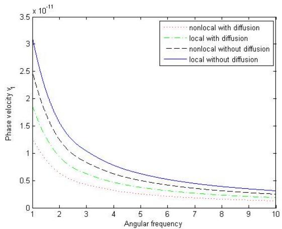Phase velocity: Figures 1-3 represent the impact of nonlocal and diffusion parameter on the phase velocities $v_{1}$, $v_{2}$ and $v_{3}$ of P-wave, T-wave, and MD-wave respectively with respect to angular frequency $\omega$. From figures 1-2, it is clear that behaviour of phase velocity of P-wave and T-wave with respect to angular frequency is same with difference in magnitude values. The phase velocities $v_{1}$ and $v_{2}$ decreases monotonically, reaches to minimum value at $\omega = 10^{0}$ for all types of thermoelastic solids. The values of $v_{1}$ and $v_{2}$ for local solid are more than that of nonlocal solid. From physical point of view, the stresses produced in nonlocal medium is weak due to impact of nano-structured particles and change in stress causes the change in wave characteristics accordingly. Also phase velocity has lower value in elastic solid with diffusion in comparison to elastic solid without diffusion. Thermoelastic waves exhibit different dispersion characteristics in thermodiffusive solid which in turn influence the Phase velocity, attenuation coefficient, penetration depth and specific loss. 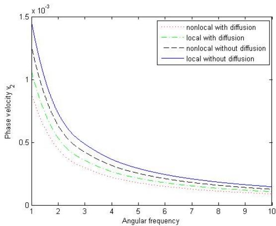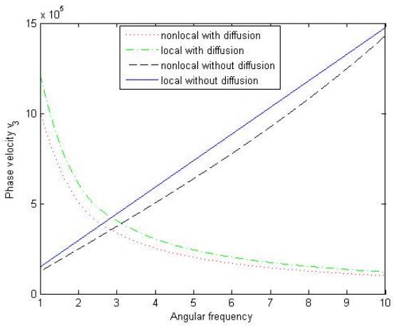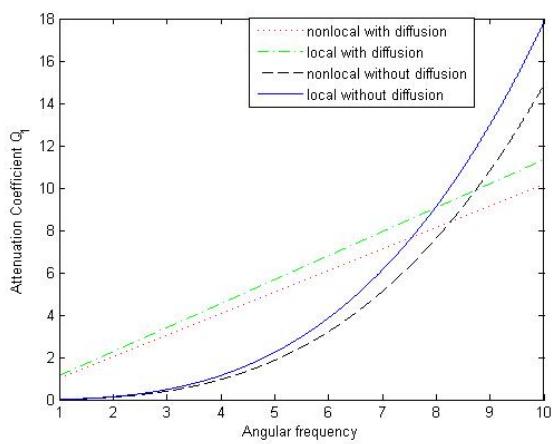Figure 3 shows that phase velocity $v_{3}$ of  Figure 1: Variation of phase velocity of P-wave   Figure 2: Variation of phase velocity of T-wave  Figure 4: Variation of attenuation coefficient of P-wave 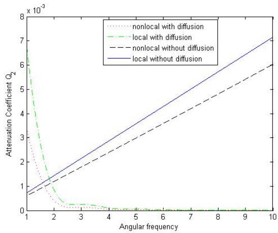 Figure 5: Variation of attenuation coefficient of T-wave MD-wave decreases monotonically reaches to minimum value at $\omega = 10^0$ for thermoelastic solid with diffusion whereas it increases linearly, reaches to maximum value at $\omega = 10^0$ for elastic solid without diffusion. Attenuation Coefficients: Figures 4-6 represent the impact of nonlocal and diffusion parameter on the attenuation coefficients $Q_{1}$, $Q_{2}$ and $Q_{3}$ of P-wave, T-wave, and MD-wave respectively with respect to angular frequency $\omega$. It has been observed from the figure 4 that attenuation coefficient $Q_{1}$ of P-wave increases parabolically for $1^{0} \leq \omega \leq 10^{0}$ in elastic solid without diffusion. For thermoelastic solid with diffusion, $Q_{1}$ increases linearly in local as well as nonlocal solid. Figure 5 shows that attenuation coefficient $Q_{2}$ of T-wave increases linearly with increase in $\omega$ in thermoelastic solid without diffusion whereas in thermodiffusive solid, it decreases sharply for $1^{0} \leq \omega \leq 2.5^{0}$. From figure 6, it is clear that attenuation coefficient $Q_{3}$ of MD-wave increases linearly in all types of solids with difference in magnitude. The value of $Q_{3}$ is lower in diffusive solid in comparison to solid without diffusion. Also, figures 4-6 show that attenuation coefficients has smaller value in nonlocal solid in comparison to local elastic solid due to nonlocal parameter. Penetration Depth: Figures 7-9 represent the effect of diffusion and non-local parameter on the penetration depth $D_{1}$, $D_{2}$ and $D_{3}$ of P-wave, T-wave, 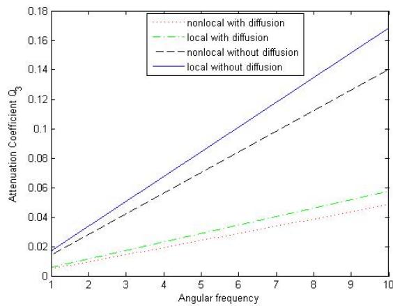 Figure 6: Variation of attenuation coefficient of MD-wave and MD-wave respectively with respect to angular frequency $\omega$. Figure 7 depicts the variation of penetration depth $D_{1}$ of P-wave with respect to angular frequency $\omega$. In thermoelastic solid without diffusion, the penetration depth $D_{1}$ decreases sharply for $1^{0} \leq \omega \leq 2.5^{0}$ and then slowly for $\omega \geq 2.5^{0}$. The value of $D_{1}$ decreases monotonically, reaches to minimum value at $\omega = 10^{0}$ in diffusive elastic solid. It has been observed from the figure 8 that penetration depth $D_{2}$ of T-wave increases in diffusive solid and decreases in solid without diffusion with increase in angular frequency $\omega$ having greater value in local solid in comparison to nonlocal elastic solid. From figure 9, it is clear that penetration depth $D_{3}$ of MD-wave decreases monotonically in all types of solids with difference in magnitude. Also, the value of $D_{3}$ is lower in diffusive solid in comparison to solid without diffusion. Specific Loss: Figures 10-12 show the effect of diffusion and nonlocal parameter on the specific loss $L_{1}$, $L_{2}$ and $L_{3}$ of P-wave, T-wave, and MD-wave respectively with respect to angular frequency $\omega$. From figures 10 and 12, it has been observed that behaviour of specific loss $L_{1}$ of P-wave is similar to behaviour of specific loss $L_{3}$ of MD-wave with difference in magnitude. Specific loss $L_{1}$ and $L_{3}$ decreases monotonically, reaches to minimum value at $\omega = 10^{0}$ in thermoelastic solid without diffusion whereas it increases linearly, reaches to maximum value at $\omega = 10^{0}$ in thermodiffusive solid. 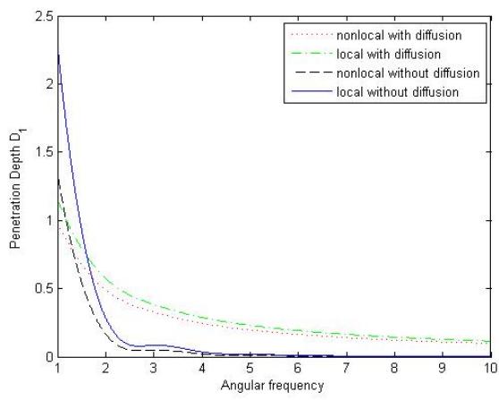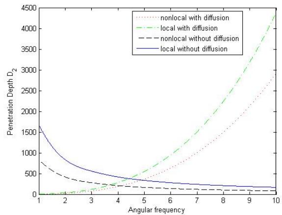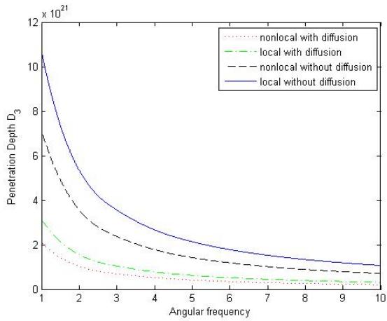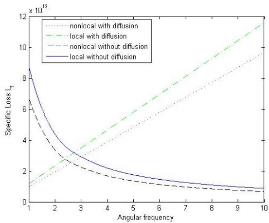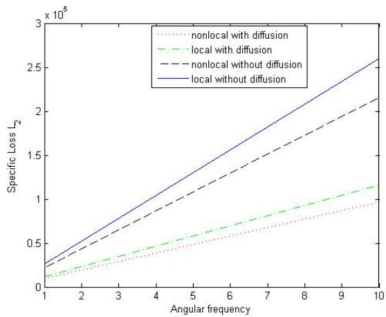Figure 11 represents the variation of specific loss $L_{2}$ of T-wave with respect to an-  Figure 7: Variation of penetration depth of P-wave  Figure 3: Variation of phase velocity of MD-wave  Figure 8: Variation of penetration depth of T-wave  Figure 9: Variation of penetration depth of MD-wave Figure 10: Variation of specific loss of P-wave  Figure 11: Variation of specific loss of T-wave 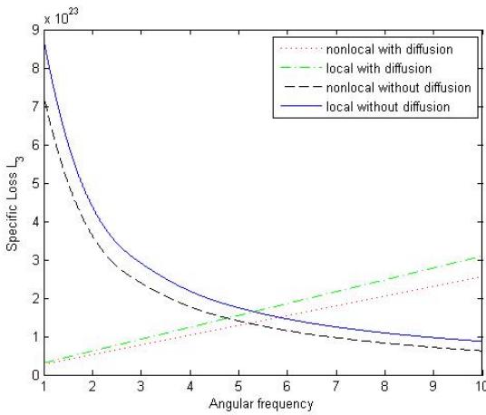 Figure 12: Variation of specific loss of MD-wave gular frequency $\omega$. In all types of solids, $L_{2}$ increases linearly, having lower value in diffusive solid as comparison to solid without diffusion. Also from figures 10-12, it is clear that specific loss has greater value in local solid as comparison to nonlocal elastic solid. ## IX. CONCLUSION We have examined the effects of nonlocal parameter on the propagation of plane wave in nonlocal homogenous isotropic thermoelastic diffusion. The major consequences of current problems are: (1) There exist three coupled waves namely P-wave, T-wave, MD-wave and one transverse wave(SV) propagating with different phase velocities. Furthermore phase velocity, attenuation coefficients, penetration depth and specific loss with respect to angular frequency are studied graphically. (2) It has been found that characteristics of all the waves are affected by diffusion and nonlocal parameter of the medium. (3) The fundamental solution of system of differential equations for steady oscillations has been constructed. (4) The analysis of fundamental solution $\mathbf{M}(\mathbf{X})$ of the system of equations (27)-(29) are helpful to investigate three dimensional problems of nonlocal homogenous isotropic elastic solid with diffusion. (5) The graphical analysis of present work is very helpful in order to investigate the various fields of aerospace, electronics and geophysics like volcanology, telecommunication etc.

Generating HTML Viewer...

References

41 Cites in Article
A Eringen (1972). Linear theory of nonlocal elasticity and dispersion of plane waves.
A Eringen (1974). Theory of nonlocal thermoelasticity.
A Eringen (1977). Edge dislocation in nonlocal elasticity.
A Eringen,D Edelen (1972). On nonlocal elasticity.
M Gurtin (1972). The linear theory of elasticity.
W Nowacki (1975). Dynamic problems of elasticity.
Witold Nowacki (1986). Theory of Micropolar Elasticity.
Albert Green,P Naghdi (1977). On thermodynamics and the nature of the second law.
Albert Green,P Naghdi (1991). A re-examination of the basic postulates of thermomechanics.
V Kupradze,T Gegelia,M Basheleishvili,T Burchuladze,E Sternberg (1979). Three-Dimensional Problems of the Mathematical Theory of Elasticity and Thermoelasticity.
Suraj Kumar,S Tomar (2020). Plane waves in nonlocal micropolar thermoelastic material with voids.
Iqbal Kaur,Kulvinder Singh (2021). Plane wave in non-local semiconducting rotating media with Hall effect and three-phase lag fractional order heat transfer.
M Aouadi (2007). Uniqueness and reciprocing theorems in the theory of generalized thermoelastic diffusion.
Moncef Aouadi (2008). Generalized Theory of Thermoelastic Diffusion for Anisotropic Media.
M Aouadi (2009). Theory of generalized micropolar thermoelastic diffusion under Lord-Shulman model.
M Aouadi (2010). A theory of thermoelastic diffusion materials with voids.
Dinesh Sharma,Dinesh Thakur,Vishal Walia,Nantu Sarkar (2020). Free vibration analysis of a nonlocal thermoelastic hollow cylinder with diffusion.
Lars Hörmander (1963). Linear Partial Differential Operators.
Lars Hörmander (1983). The Cauchy problem (constant coefficients).
R Hetnarski (1964). The fundamental solution of the coupled thermoelastic problem for small times.
Richard Hetnarski (1964). Coupled Problem of Thermoelasticity: Solution in a Series of Functions Form.
W Svanadze (1988). The fundamental matrix of linearized equations of the theory of elastic mixtures.
M Svanadze (1996). THE FUNDAMENTAL SOLUTION OF THE OSCILLATION EQUATIONS OF THE THERMOELASTICITY THEORY OF MIXTURE OF TWO ELASTIC SOLIDS.
Merab Svanadze (2004). FUNDAMENTAL SOLUTIONS OF THE EQUATIONS OF THE THEORY OF THERMOELASTICITY WITH MICROTEMPERATURES.
Merab Svanadze (2004). Fundamental solution of the system of equations of steady oscillations in the theory of microstretch elastic solids.
E Scarpetta (1990). The fundamental solution in micropolar elasticity with voids.
M Ciarletta,A Scalia,M Svanadze (2007). Fundamental solution in the theory of micropolar thermoelasticity for materials with voids.
Merab Svanadze,Vincenzo Tibullo,Vittorio Zampoli (2006). Fundamental Solution in the Theory of Micropolar Thermoelasticity without Energy Dissipation.
R Kumar,T Kansal (2004). Fundamental solution in the generalized theories of thermoelastic diffusion.
Rajneesh Kumar,Tarun Kansal (2012). Fundamental solution in the theory of micropolar thermoelastic diffusion with voids.
K Sharma,P Kumar (2013). Propagation of plane waves and fundamental solution in thermoviscoelastic medium with voids.
Rajneesh Kumar,Krishan Kumar,Ravendra Nautiyal (2013). Plane waves and fundamental solution in a couple stress generalized thermoelastic solid.
Rajneesh Kumar,Mandeep Kaur,S Rajvanshi (2015). Representation of Fundamental and Plane Waves Solutions in the Theory of Micropolar Generalized Thermoelastic Solid with Two Temperatures.
Rajneesh Kumar,Shaloo Devi (2016). Plane waves and fundamental solution in a modified couple stress generalized thermoelastic with three-phase-lag model.
S Biswas (2019). Fundamental solution of steady oscillations for porous materials with dual-phase-lag model in micropolar thermoelasticity.
R Kumar,D Batra (2020). Fundamental solution of steady oscillations in swelling porous thermoelastic medium.
Siddhartha Biswas (2020). Fundamental solution of steady oscillations equations in nonlocal thermoelastic medium with voids.
Siddhartha Biswas (2021). The propagation of plane waves in nonlocal visco-thermoelastic porous medium based on nonlocal strain gradient theory.
R Kumar,S Ghangas,A Vashishth (2021). Fundamental and plane wave solution in non-local bio-thermoelasticity diffusion theory.
Poonam,Ravinder Sahrawat,Krishan Kumar (2021). Plane wave propagation and fundamental solution in non-local couple stress micropolar thermoelastic solid medium with voids.
R Kumar,D Batra (2022). Plane wave and fundamental solution in steady oscillation in swelling porous thermoelastic medium.
No ethics committee approval was required for this article type.
Data Availability
Not applicable for this article.
How to Cite This Article
Krishan Kumar. 2026. \u201cPlane Wave Propagation and Fundamental Solution for Nonlocal Homogenous Isotropic Thermoelastic Media with Diffusion\u201d. Global Journal of Science Frontier Research - F: Mathematics & Decision GJSFR-F Volume 23 (GJSFR Volume 23 Issue F3): .
Explore published articles in an immersive Augmented Reality environment. Our platform converts research papers into interactive 3D books, allowing readers to view and interact with content using AR and VR compatible devices.
Your published article is automatically converted into a realistic 3D book. Flip through pages and read research papers in a more engaging and interactive format.
In the present problem, we study plane wave propagation and establish fundamental solution in the theory of nonlocal homogenous isotropic thermoelastic media with diffusion. We observe that there exists a set of three coupled waves namely longitudinal wave(P), thermal wave(T) and mass diffusion wave(MD) and one uncoupled transverse wave(SV) with different phase velocities. The effects of nonlocal parameter and diffusion on phase velocity, attenuation coefficient, penetration depth and specific loss have been studied numerically and presented graphically with respect to angular frequency. It is observed that characteristics of all the waves are influenced by the diffusion and nonlocal parameter. Fundamental solution of differential equations of motion in case of steady oscillations has been investigated and basic properties have also been discussed. Particular case of interest is also deduced from the present work and compared with the established result.
Our website is actively being updated, and changes may occur frequently. Please clear your browser cache if needed. For feedback or error reporting, please email [email protected]
Thank you for connecting with us. We will respond to you shortly.