## I. INTRODUCTION Mathematics is an essential tool for data processing in all natural sciences, including chemistry [1-4]. However, in all of them, there are several stereotypes of presenting different mathematical equations. Most of them are the following: in equations of the form $y = f(x, \ldots)$ the argument(s) (x, ...) are typically on the right side, while the function is on the left. The number of possible examples is so large that it is difficult to estimate it. For instance, the well known Antoine equation which has many chemical applications relates the absolute temperature $(T,$ argument), and the vapor pressure of pure liquids $(P,$ function): $\log P = a / T + b$ (the coefficients $a$ and $b$ should be precalculated). If necessary, the argument and function can be swapped and this relationship can be used to calculate the temperature from the pressure. Besides that numerous analogues of Antoine equation are used in different areas. For instance, the dependence of retention times vs. temperature of gas chromatographic column is described with Antoine-like equation $\log (t_{\mathrm{R}}^{\prime}) = a / T + b$. Numerous other forms of representing dependences (e.g., parametric) are known for mathematicians, but in chemistry they are perceived as rather unusual. Recurrent equations are precisely such unusual forms of mathematical relationships. The main feature of them is the absence of arguments in their writing: recurrent equations relate the current value of a function to its previous value(s). The rare use of these relations is confirmed by the fact that many contemporary manuals have no information about them. Recurrent (recursive) progressions are mentioned in [2, P. 174] only as a particular case for comparing with other progressions (arithmetic, geometric, etc.). Such an attitude towards recurrences cannot be accepted, since the properties of recurrences make them indispensable mathematical object in chemistry. The main reason of that is, probably, just unusual mathematical form of recurrences, namely the absence of arguments. The purpose of this article is to illustrate the application of recurrences with examples from various areas of chemistry and chromatography. Generally, the most straightforward (first-order) linear recurrences can be represented in two ways. The first kind of recurrence combines the values of functions of discrete integer arguments $(n + 1$ and $n)$ in relation (1): $$ y (n + 1) = a y (n) + b \tag {1} $$ The coefficients $a$ and $b$ should be precalculated by the least-squares method using data for a preselected training set. At first glance, the scope of application of such relations with integer arguments seems to be somewhat limited. However, it is not; in organic chemistry many properties of organic compounds are considered as the functions of their positions in the corresponding homologous series, or, in other words, of the number of carbon (or other elements) atoms in the molecule. Meanwhile, the number of atoms of any element in a molecule can take integer values only. It is the principal reason for the applying of recurrent dependences to various properties of organic compounds. One can only be surprised that this was not been done before 2006, but it may only be explained by the unfamiliarity of these relations. The second form of recurrent dependences applies to any functions for which it is possible to provide the equidistant argument values, namely, in the form $(x + \Delta x)$, where $\Delta x = \text{const}$ (relation 2). In other words, the experimenter must select appropriate argument values from their possible multitude: $$ y(x + \Delta x) = a y(x) + b, \Delta x = \mathrm{const} $$ Such an expansion of the domain of definition allows applications of recurrences to functions of continuous variables such as temperature $(T)$, pressure $(P)$, concentrations $(C)$, etc., i.e., not only to properties of homologs in organic chemistry, but also to characteristics of chemical systems in physical, analytical, inorganic chemistry, etc. The general feature of recurrences is the absence of argument values in both parts (left and right) of equalities. Every point on the plots of recurrences is specified by two values of functions: current and previous, or current and subsequent ones. The second feature of equation (2) is the appearance of the additional (artificial) variable $\Delta x$: the shape of the graph begins to depend on this value. 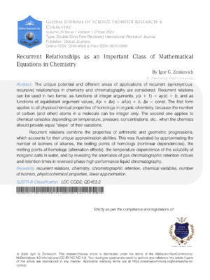As a result, both forms of recurrences are somewhat difficult to visualize, which explains in some way their rare use in scientific practice. To illustrate this, let us consider as an example the recurrent representation of any well-known function $y(x)$. Let us select 36 points within the domain of its definition with the increment $\Delta x = 10$ and build a plot corresponding to the equation $y(x + 10) = ay(x) + b$, shown in Fig. 1. 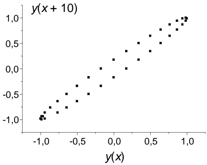 Fig. 1: Recurrent representation of a well-known mathematical function in the form $y(x + 10) = ay(x) + b$. It is not so easy to recognize it We obtain some kind of closed ellipsoidal curve, which has no analogues among the plots of commonly used functions. If we change the value $\Delta x$ and select $\Delta x = 1$ (or less) instead of $\Delta x = 10$, the ellipsoidal curve will turn into a practically straight segment located between points $(-1, -1)$ and $(+1, +1)$. So as not to continue the intrigue, let us note that this function is $y = \sin x$, but it is rather difficult to "recognize" it from the recurrent graph without special preparation. First-order recurrent relations like (1) or (2) look like simple mathematical expressions only at a first glance. These equations have the non-recurrent algebraic solution that is an unusual type of polynomial of variable degree, because the values of the argument are the power: $$ y (x) = y (0) a ^ {x} + b \left(a ^ {x} - 1\right) / (a - 1) \tag {3} $$ This solution can be easily found using MAPLE software. The value of the auxiliary parameter $y(0)$ should be predetermined, for example, using the value $y(1)$, because at $x = 1$ $y(1) = y(0)a + b$, and $y(0) = [y(1) - b] / a$. This solution is the row, because $(a^x - 1) / (a - 1) = a^{x-1} + a^{x-2} + \ldots + 1$. The variable degree of this polynomial is a crucial explanation of the usefulness of   applying recurrences to approximation of chemical variables. This fact deserves special comments. Example 1: Let us try to approximate the nonlinear dependence of normal boiling points of 1-chloroalkanes $\mathrm{C}_n\mathrm{H}_{2n + 1}\mathrm{Cl}$ on the number of carbon atoms in a molecule: $46.2^{\circ}\mathrm{C}$ $(n = 3)$, $78.4^{\circ}\mathrm{C}$ $(n = 4)$, $107.8^{\circ}\mathrm{C}$ $(n = 5)$, $135.6^{\circ}\mathrm{C}$ $(n = 6)$, $160.6^{\circ}\mathrm{C}$ $(n = 7)$, $183.8^{\circ}\mathrm{C}$ $(n = 8)$, $205.4^{\circ}\mathrm{C}$ $(n = 9)$, and so on. The commonly used way to do this is choosing the fixed-degree polynomial (e.g., second or third). At the same time, the polynomial of variable degree (3) will have the degree $x = 3$ for propyl chloride $(n = 3)$, $x = 4$ for butyl chloride $(n = 4)$, $x = 5$ for pentyl chloride $(n = 5)$, etc. In addition, a noticeable consequence of the application of this approach can be derived from this solution. If $a \equiv 1$ and $b \neq 0$, equation (3) transforms into the relation for a simple arithmetic progression, $y(x) = k + bx$. At the same time, if $0 < a \neq 1$ and $b \equiv 0$, this equation transforms into the expression for geometric progression, $y(x) = ka^x$. Hence, in the general case (at arbitrary values of coefficients $a$ and $b$ ), the recurrent equation (1) and/or (2) combines the mathematical properties of both kinds of progressions in variable proportions. It explains us the excellent approximating "power" of recurrences for numerous chemical variables. Thus, we must conclude that recurrences are not the particular case of other progressions [2] but are their generalization. The second noticeable consequence from equation (3) is the behavior of function $y(x)$ or $A(n_{\mathrm{C}})$ with a hypothetical increase in the number of carbon atoms in a molecule, $x \to \infty$, or $n_{\mathrm{C}} \to \infty$. If the value of coefficient $a$ obeys the inequality $a < 1$, the limit of polynomial (3) exists, and it is equal to: $$ \left. \lim A \left(n _ {\mathrm {C}}\right)\right| _ {\mathrm {n C} \rightarrow \infty} = b / (1 - a) \tag {4} $$ If $a > 1$, the initial numerical sequence has no limit and tends to infinity. The author cannot cite all his papers devoted to the properties and chemical applications of recurrences due to the necessity to restrict the self-citation. Only six of them published within the period from 2009 to 2024 are mentioned as references [5-10]. To conclude the Introduction, it should be noted that, probably, the most famous and widely mentioned examples of recurrences are so-called Fibonacci numbers, $F_{n}$, known since ancient times \[11-13\]: $$ F_{n}=F_{n-2}+F_{n-1},\quad(F_{0}=F_{1}=1)\tag{5} $$ A special journal named *The Fibonacci Quarterly* has been published since 1963 (see ref. [11]). ## II. EXPERIMENTAL This semi-review article does not imply specific experimental conditions. The necessary data are available from the references cited. In general, recurrent relationships can be applied to any non-linear set of equidistant variables not only in chemistry or chromatography. For example, the temperatures of the cooling kettle, $T(^{\circ}\mathrm{C}) = f(t,\min)$ are: 72(0), 62(5), 55(10), 50(15), 46(20), etc. All these data correspond to the linear recurrent dependence $T(t + 5\min) = aT(t) + b$ with the following parameters: $a = 0.72 \pm 0.01$. $b = 10.0 \pm 0.8$, $R = 0.9996$, $S_0 = 0.2$. Another important example is the approximation of the carbon dioxide content in the atmosphere of Earth (data from site http://climate.gov), $(\mathrm{CO}_{2}$ concentration (ppm)) $= f(\text { year })$: 324(1970), 337(1980), 353(1990), 369(2000), 390(2010), and 412(2020). Parameters of the recurrence $C(\text { year } + 10) = a C(\text { year }) + b$ are: $a = 1.14 \pm 0.01, b = -33 \pm 8, R = 0.9994, S_{0} = 1.2$. After that we can easily (because the dependence is linear) estimate the concentration of $\mathrm{CO}_{2}$ in the atmosphere at 2030: it should be $1.14 \times 412 - 33 = 437 \text { ppm }$. The values of different physicochemical properties of organic compounds (boiling points, melting points, etc.) were taken from all available sources of reference information, e.g., [14], as well as from Internet. The necessary stage of processing the initial information was the rejection of outliers, followed by averaging the data. It is required because recurrences are very "sensitive" even to minor errors in data sets. The simplicity of recurrent calculations requires special comments. The use of, e.g., Origin software implies the following stages. First, the initial data on the function of integer (equation 1) or equidistant (equation 2) arguments are entered into column A[X]. The next step is copying all data from this column excluding the value from the first line into column B[Y] with shifting one line up. Just such shifting is the sense of recurrences. After that, we can operate with the obtained two-dimensional data array in the usual way, i.e., plot this dependence and calculate all the parameters of the linear regression $y(x + 1) = ay(x) + b$. For example, let us make the recurrent approximation of the squares of natural numbers from 3 to 10. Hence, the first column (Origin or Excel software) contains the values 9, 16, 25, 36, 49, 64, 81, and 100 (eight values). The second column (shifted) in the same lines contains the values 16, 25, 36, 49, 64, 81, and 100. In the result we obtain seven pairs of numbers for calculating the parameters of linear regression by least squares method: $a = 1.16 \pm 0.01$, $b = 4.5 \pm 0.5$, $R = 0.9998$, $S_0 = 0.7$. The plot of this dependence looks like "ideal" straight line. Such calculations are very simple, and the application of no special functions is required. ## III. RESULTS AND DISCUSSION ### a) Chemical Applications ## i. Number of Isomers In this section, it seems advisable to avoid considering the simplest artificial examples and start directly with real chemical problems. The first is the dependence of the number of structural isomers $(N)$ of homologs on the number of carbon atoms in their molecules $(n_{\mathrm{C}})$. The number of such isomers for $n$ -alkanes $\mathrm{C}_{5}-\mathrm{C}_{18}$ is listed in Table 1; it is the rapidly increasing function [15]. It is noteworthy that estimates of the number of isomeric alkanes with $n_{\mathrm{C}} = 18$ and above, obtained by different methods, appeared to be slightly different, e.g., 60524 vs. 60523 for $\mathrm{C}_{18} \mathrm{H}_{38}$. However, such small differences for many practical purposes are negligible. Table 1: Number of structural isomers of alkanes ${\mathrm{C}}_{\mathrm{n}}{\mathrm{H}}_{2\mathrm{n} + 2}$ <table><tr><td>Number of Carbon Atoms, Nc</td><td>Number of Structural Isomers, N</td><td>Log n</td></tr><tr><td>5</td><td>3</td><td>0.477</td></tr><tr><td>6</td><td>5</td><td>0.699</td></tr><tr><td>7</td><td>9</td><td>0.954</td></tr><tr><td>8</td><td>18</td><td>1.255</td></tr><tr><td>9</td><td>35</td><td>1.544</td></tr><tr><td>10</td><td>75</td><td>1.875</td></tr><tr><td>11</td><td>159</td><td>2.201</td></tr><tr><td>12</td><td>305</td><td>2.550</td></tr><tr><td>13</td><td>802</td><td>2.904</td></tr><tr><td>14</td><td>1858</td><td>3.269</td></tr><tr><td>15</td><td>4347</td><td>3.638</td></tr><tr><td>16</td><td>10359</td><td>4.015</td></tr><tr><td>17</td><td>24894</td><td>4.396</td></tr><tr><td>18</td><td>60524 (60523)*</td><td>4.782</td></tr></table> The plot of this function $N = f(n_{\mathrm{C}})$ for alkanes with $5 \leq n_{\mathrm{C}} \leq 17$ is presented in Fig. 2(a). It seems rather challenging to precalculate the number of isomeric alkanes with a higher number of carbon atoms because we do not know the type of this function (it should be evaluated or assumed preliminarily). However, if we transform this dependence to the linear form, the problem's solution enormously simplifies, because we can evaluate other values using the simplest linear extrapolation. Just recurrent approximations allow us to implement this approach.  (a) 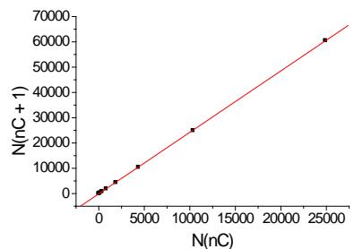 (b) 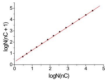 (c) Fig. 2: (a) Plot of the number of structural isomers of alkanes $\mathsf{C}_n\mathsf{H}_{2n + 2}$ (N) vs. the number of carbon atoms in the molecule $(n_c)$; (b) plot of the recurrent dependence $N(n_{c} + 1) = aN(n_{c}) + b$; parameters of the linear regression: a $= 2.429\pm 0.004$ b $= -62\pm 30$ R $= 0.99999$ $\mathsf{S}_0 = 98$ c plot of the recurrent dependence of logarithms, $\log N(n_{c}+$ $1) = \mathrm{alog}N(n_{c}) + \mathrm{b};$ parameters of the linear regression: a $= 1.036\pm 0.005$ b $= 0.248\pm 0.012$ R $= 0.9998$ $\mathsf{S}_0 =$ 0.02 Approximating the data set in the form $N(n_{\mathrm{c}} + 1)$ vs. $N(n_{\mathrm{c}})$ gives the plot presented in Fig. 2(b). It is a linear dependence with the correlation coefficient $R = 0.99999$. Other parameters of the linear regression are indicated in the footnote to Fig. 2. If the correlation coefficients exceed 0.999, the plots of such dependencies are visually perceived as absolutely straight lines. It is an essential moment in the characterization of recurrent dependencies. For numerous chemical variables, these dependencies are linear, but if not, the reasons of deviations from linearity should be investigated. If we will use this result for evaluating the number of isomers of alkane $\mathsf{C}_{18}\mathsf{H}_{38}$ using the number of isomers for the previous alkane $\mathsf{C}_{17}\mathsf{H}_{36}$, we should make the following simple calculations: $$ 24894\times2.429-62\approx60406 $$ For the example considered the evaluation of uncertainty appeared to be approximately $\pm 98$. The correct answer is 60524 or 60523 isomers (Table 1). Hence, the relative error is approximately $0.19\%$. Such accuracy seems to be enough for many practical purposes. This example illustrates another feature of recurrent approximation. If it is linear for variable $x$, it remains linear for any monotonic functions of this variable, e.g., $x^n$, $\log(x)$, $\exp(x)$, etc. Hence, we can approximate not the number of isomeric alkanes $(N)$ but  (a) (c)  $T_{\mathrm{b}}(n_{\mathrm{C}})$, ${}^{\circ}\mathbf{C}$ the log $N$ values. Fig. 2(c) illustrates the linear recurrent dependence for logarithms of isomers' number. The number of isomers of homologs of other series [16, 17] can be approximated using recurrent relations without any restrictions. ## ii. 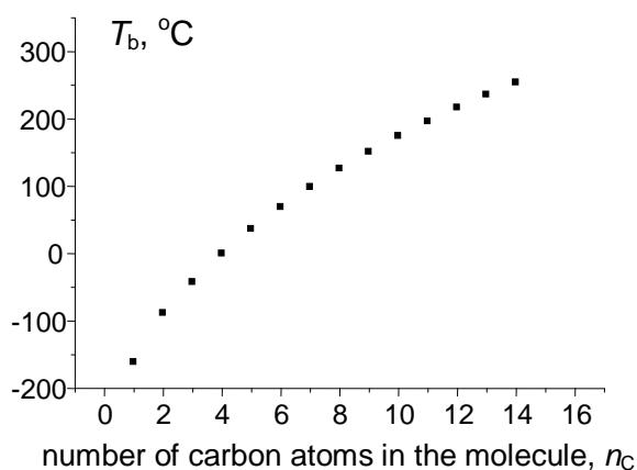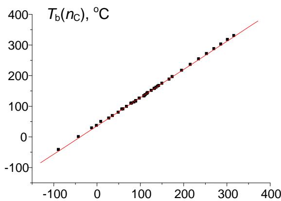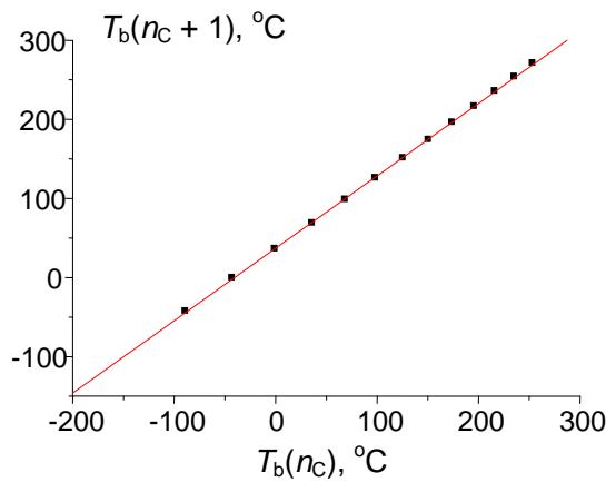Approximation of Boiling Points of Homologs To illustrate the potential of recurrent relations in form (1) (functions of integer argument), let us consider the approximation of values of any physicochemical properties of homologs. The simplest example is normal (at the atmospheric pressure) boiling points $(T_{\mathrm{b}})$ of $n$ -alkanes $\mathsf{C}_n\mathsf{H}_{2n + 2}$ within the set of compounds $\mathsf{C}_2 - \mathsf{C}_{14}$ (if necessary, this range can be expanded); the reference data are readily available [14]. The plot in Fig. 3(a) illustrates the initial nonlinear dependence $T_{\mathrm{b}}(n_{\mathrm{C}})$; the linear recurrent approximation $T_{\mathrm{b}}(n_{\mathrm{C}} + 1) = aT_{\mathrm{b}}(n_{\mathrm{C}}) + b$ is illustrated in Fig. 3(b). The parameters of the linear regression are listed in the footnote to this figure.  (b) 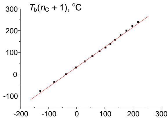 (d) $T_{\mathrm{b}}(n_{\mathrm{C}})$, ${}^{\circ}\mathbf{C}$ Fig. 3: (a) Dependence of the normal boiling points of n-alkanes $C_1 - C_{14}$ ( $^\circ C$ ) on the number of carbon atoms in the molecule; (b) recurrent approximation of the normal boiling points (equation 1); parameters of linear regression: $a = 0.916 \pm 0.003$, $b = 36.9 \pm 0.5$, $R = 0.99993$, $S_0 = 1.2$; (c) recurrent approximation of the normal boiling points for all alkanes (including branched isomers); parameters of the linear regression: $a = 0.922 \pm 0.003$, $b = 35.6 \pm 0.5$, $R = 0.9997$, $S_0 = 2.0$; (d) recurrent approximation of the normal boiling points for perfluoro-1-alkanes $C_nF_{2n+2}$; parameters of the linear regression: $a = 0.91 \pm 0.01$, $b = 32.5 \pm 1.4$, $R = 0.9991$, $S_0 = 4.2$ The next exciting feature of recurrences does not follow from their mathematical properties but has a critical chemical sense. Namely, if the recurrent linearization is valid for normal alkanes (with nonbranched carbon skeleton), the equation with practically the same coefficients will be valid for all isomeric structures of the same class, i.e., for alkanes with branched carbon skeletons. It is illustrated by Fig. 3(c) (39 points for iso-alkanes were added). Comparing the coefficients of recurrences (b) and (c) confirm their identity: 0.916 and 0.922 (values of coefficient $a$ ), as well as 36.9 and 35.6 (values of coefficients $b$ ). Moreover, combining the data for 189 homologs of 10 different homologous series confirms the existence of a single linear relationship for all of them with the following parameters: $a = 0.930 \pm 0.002$, $b = 33.5 \pm 0.3$, $R = 0.9995$, $S_0 = 2.4$ [7]. It allows us to conclude that coefficients $a$ and $b$ or recurrent regressions are close to each other for all homologous series with the same homologous differences, at first $\mathrm{CH}_2$. The following example illustrates the applicability of recurrences not to alkanes but compounds of other chemical nature. The plot of the recurrent approximation of boiling points of perfluoro- $n$ -alkanes $\mathsf{C}_1 - \mathsf{C}_{14}$ is presented in Fig. 3(d). The correlation coefficient of this dependence exceeds 0.999. The linearity of recurrent relations makes it possible to evaluate the boiling points of any next homologs using the data for previous ones. Example 2: Let us evaluate the normal boiling point of 1-chlorodecane using $T_{\mathrm{b}}$ value for 1-chloronone (205.4°C, see Example no. 1). The values of recurrent coefficients for the series of chloroalkanes are $a = 0.923 \pm 0.002$, $b = 35.7 \pm 0.3$, $R = 0.99999$, and $S_{0} = 0.3$. The next step of calculations is simple: $205.4 \times 0.923 + 35.7 = 225.3^{\circ}\mathrm{C}$ (the reference value is $225.8^{\circ}\mathrm{C}$ ). Example 3: Let us evaluate the normal boiling point of $n$ -butylisocyanate using $T_{\mathrm{b}}$ value for $n$ -propylisocyanate (88°C). As the data for the series of alkyl isocyanates are insufficient to calculate the coefficients of equation (1), let us use the "universal" values of these coefficients for any homologous series (see above). The result is $88 \times 0.930 + 33.5 = 115.6^{\circ}\mathrm{C}$ (the reference value is $115^{\circ}\mathrm{C}$ ). Recurrent relations provide linear approximations of not only normal boiling points but also the values of other physicochemical properties of organic compounds within homologous series, $A(n_{\mathrm{C}})$. These include, for example, relative density $(d_4^{20})$, refractive index $(n_{\mathrm{D}}^{20})$, dynamic viscosity $(\mu)$, surface tension $(\sigma)$, ionization potential $(I)$, acidity constant $(pK_{a})$, dielectric permittivity $(\varepsilon)$, water solubility $(w, pS)$, and many others. The fundamental requirement to the dependences $A(n_{\mathrm{C}})$ is the same: these functions should be monotonic (the signs of their first derivatives should be constant). The example of nonmonotonic dependencies is, for instance, the temperature dependence of the solubility of organic compounds in water. Due to the problem of the monotony of changes in the values of physicochemical properties of organic compounds, it is interesting to consider another form of recurrent relations, namely, second-order recurrences: $$ y (n + 2) = a y (n) + b \tag {5} $$ ## iii. Melting Points of Homologs Similarly to the previous ones, the coefficients $a$ and $b$ of equation (5) should be precalculated by the least-squares method. The algebraic solution of equation (5) can be found in the same way as the solution of equation (1) using MAPLE software. 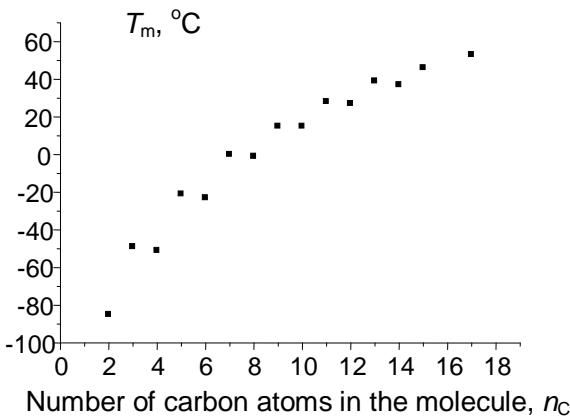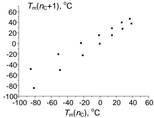Surprisingly, it turned out to be much more complex than the solution of (1): $$ y(x) = \frac{(y(0)a - y(1))\sqrt{a}(-\sqrt{a})\uparrow x - (y(1)\sqrt{a} - a y( 0)) (\sqrt{a})\uparrow x}{2a} - \frac{b}{a - 1} - \frac{b(\sqrt{a} - a)(-\sqrt{a})\uparrow x + b(\sqrt{a} + a)(\sqrt{a})\uparrow x}{2a(a - 1)} \tag{6} $$ Relation (6) obviously cannot be recommended for any calculations due to its complexity, but it allows us to make important conclusions. First, this solution contains negative terms to the $x$ power, namely (-sqr(a)) $\uparrow x$. It means that these terms have different signs depending on whether the $x$ -values are even or odd. Therefore, the presence of terms with alternating signs in the equation makes it applicable for approximation of variables with pronounced alternation effects. The most important of these variables are the melting points of homologs with even and odd numbers of carbon atoms in the molecules. The alternation of the melting point is well known for $n$ -alkanes, $n$ -alkenes, 1-alkanols, carboxylic acids, 1-alkylamines, numerous 1,ω- difunctionalized alkanes, etc. Fig. 4 illustrates different kinds of the recurrent data approximation for 1-alkylamines. Plot (a) represents the set of initial data, "distorted" with alternation effects. The first-order linear recurrent approximation (equation 1) converts this plot to two nonparallel straight lines (b). Finally, the application of equation (5) to this data set gives a single straight line with the correlation coefficient $R = 0.9996$ (no less than the $R$ -values in the other cases mentioned above), but with irregular arrangement of points (c). The parameters of linear regression (c) are listed in the footnote.  (a)  (b) 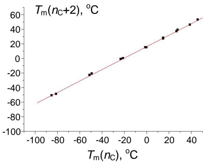 (c) Fig. 4: (a) Dependence of the melting points of n-alkylamines $\mathrm{C}_2 - \mathrm{C}_{18}$ ( $^\circ\mathrm{C}$ ) on the number of carbon atoms in the molecule; the alternation effect is easily noticeable; (b) recurrent approximation of the melting points (equation 1); all points belong to two non-parallel lines; (c) recurrent approximation of the melting points for n-alkyl amines (equation 4); parameters of the linear regression: $a = 0.786 \pm 0.006$, $b = 16.1 \pm 0.2$, $R = 0.9996$, $S_0 = 0.9$ Secondly, despite the complexity of equation (6), it is easy to conclude that the limiting value of $y(x)$ at $x \to \infty$ is the same as that of the polynomial (3), namely, $b / (1 - a)$. Hence, we can evaluate the melting point for hypothetical 1-alkylamine with $n_{\mathrm{C}} = \infty$, i.e., $16.1 \times (1 - 0.786) \approx 75^{\circ} \mathrm{C}$. The highest-molecular-mass 1-alkylamine for which the melting point has been determined is 1-octadecylamine with $T_{\mathrm{m}} 53^{\circ} \mathrm{C}$ [14]. Another example with alternating melting points of homologous $n$ -alkane carboxylic acids is considered in [5]. ## iv. 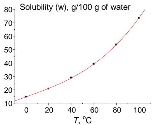Temperature Dependence of Solubility of Inorganic Salts in Water The next possible application of recurrences is approximating the temperature dependence of the solubility of inorganic salts in water, $w(7)$, $g / 100 \, \text{g}$ of water. It is known that numerous inorganic and some organic compounds form hydrates in aqueous solutions. Using the recurrences allows us to detect important features of the data sets on solubility, namely, the formation of hydrates. If the dissolved compound exists in the single chemical form (either hydrated or non-hydrated) at different temperatures of the solution, the recurrent approximation of $w(T)$ dependence has no anomalies; i.e., it is linear. This case can be illustrated with plots for the solubility of copper sulfate within the temperature range $0 \leq w(T) \leq 100^{\circ}\mathrm{C}$ presented in Fig. 5. Despite the nonlinearity of the initial dependence $w(T)$ (a), its recurrent approximation has the correlation coefficient $R = 0.9998$ (b).  (a) 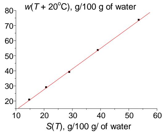 (b) Fig. 5: (a) Nonlinear temperature dependence of the solubility of copper sulfate pentahydrate $(\mathrm{CuSO}_4 \cdot 5\mathrm{H}_2\mathrm{O})$; (b) linear recurrent approximation of this dependence, $w(T + 20^{\circ}\mathrm{C}) = aw(T) + b$; parameters of the linear regression: $a = 1.36 \pm 0.02$, $b = 0.4 \pm 0.6$, $R = 0.9998$, $S_0 = 0.5$ Another example is the solubility of potassium acetate (Fig. 6). Considering the initial $w(T)$ dependence (a) does not allow us to decide whether the leftmost point is weird or belongs to a general nonlinear dependence. The red line in plot 6(a) results from approximation $w(T)$ by a fourth-degree polynomial. However, if we present the same data in the recurrent form, we obtain the linear dependence for all the points $(R = 0.9998)$, excluding the leftmost one, which is an obvious outlier. It follows from this fact that, at low temperatures (e.g., $0^{\circ}\mathrm{C}$ ), this salt exists in another form, less soluble than we can expect from the dependence $w(T)$ at other temperatures. 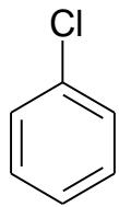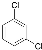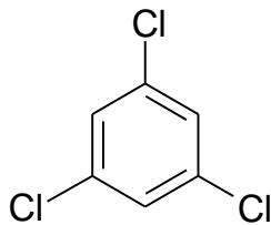### b) Applications of Recurrences in Chromatography ## i. 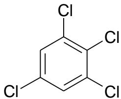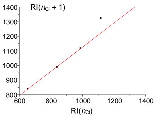Revealing the anomalies of gas chromatographic retention indices of chlorinated benzenes Gas chromatographic retention indices (RI) are important chromatographic characteristics of analytes  (I)  (II)  (III)  (IV)  (V) RI values on standard non-polar polydimethylsiloxane stationary phases \[18\]: $$ 6 5 4 \pm 7 $$ $$ 8 3 9 \pm 7 $$ $$ 9 8 9 \pm 1 0 $$ $$ 1 1 1 7 \pm 1 4 $$ $$ 1 3 2 2 \pm 1 1 $$ Adding the next chlorine atom (1,2,3,5-tetrachlorobenzene, V) will cause it to be in an ortho-position to two other chlorine atoms, which gives rise to steric tension in the molecule. However, it is difficult to identify this effect directly from the dependence $\mathrm{RI} = f(n_{\mathrm{Cl}})$ (Fig. 7(a)). At first glance, only the second point from the right on this plot seems to be located slightly below the regression line, which is not understandable. At the same time, plotting the recurrent dependence $\mathrm{RI}(n_{\mathrm{Cl}} + 1) = a\mathrm{RI}(n_{\mathrm{Cl}}) + b$ (Fig. 7(b)) immediately reveals the anomaly just for the rightmost point corresponding to tetrachlorobenzene (V). The steric hindrance in this tetrachlorobenzene increases its retention index above the value extrapolated from data for other (non-  hindered) congeners. Similar effects are also observed for retention indices of bromo- and methyl-substituted benzenes. 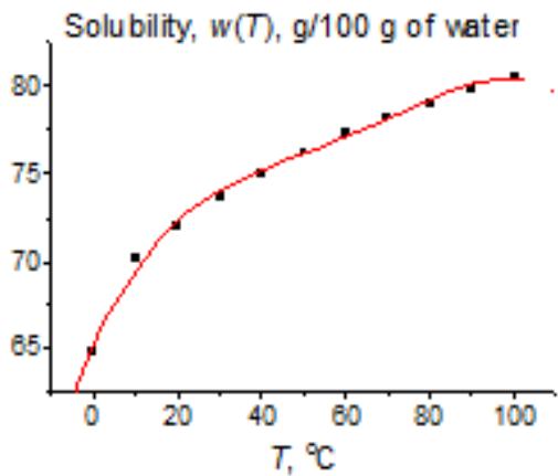 (a) 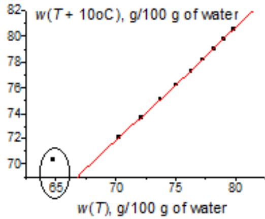 (b) Fig. 6: (a) Nonlinear temperature dependence of the solubility of potassium acetate $(\mathrm{CH}_3\mathrm{CO}_2\mathrm{K})$ in water; (b) recurrent approximation of this dependence, $w(T + 10^{\circ}\mathrm{C}) = aw(T) + b$; parameters of the linear regression without the leftmost point: $a = 0.882 \pm 0.005$, $b = 10.1 \pm 0.4$, $R = 0.9998$, $S_0 = 0.5$. 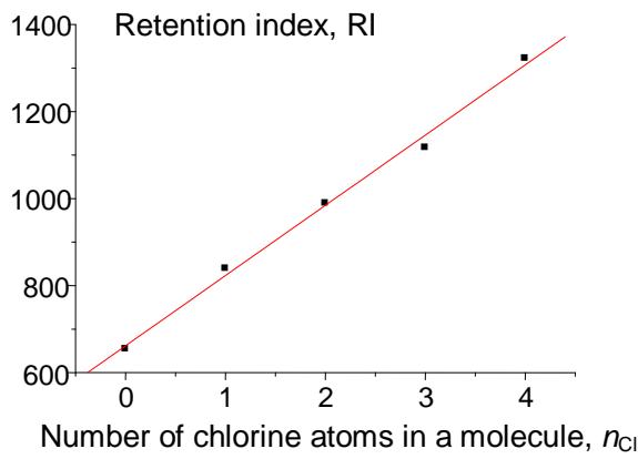 (a)  (b) Fig. 7: (a) Dependence of the retention indices of benzene and its four chloroderivatives (see text) on the number of chlorine atoms (standard nonpolar polydimethylsiloxane stationary phase); (b) recurrent approximation of this dependence, $RI(n_{Cl} + 1) = aRI(n_{Cl}) + b$; parameters of the linear regression without the rightmost point: $a = 0.83 \pm 0.01$, $b = 296 \pm 10$, $R = 0.9998$, $S_0 = 2.9$ The last example illustrates the next important feature of recurrences. In many cases, the deviations of recurrent approximations from the linearity seem to be no less informative than the linearity of these dependencies. The explanation of this fact appears to be relatively simple: Recurrent relations (1) or (2) allow linear approximations of numerous monotonic dependencies, but preferably if they can be described with a single equation. If these dependencies are distorted by additional effects, the high "linearization ability" of recurrences appeared to be insufficient for their linearization. This feature allowed us to detect the steric effects of the fourth chlorine atom in RI values of chlorinated benzenes. ## ii. Revealing the anomalies of retention parameters in reversed-phase high-performance liquid chromatography Considering the results of the last example, let us discuss the unusual applications of recurrent relations in reversed-phase high-performance liquid chromatography (RP HPLC). It is the contemporary analytical method based on the different distribution of smallest amounts of analyzed compounds (analytes) between moving liquid phase (eluent) and stationary phase fixed in a chromatographic column (modified silica gels). The dependences of retention times of analytes on the content of organic solvent in an eluent, $t_{\mathbb{R}}(C)$, should be considered first. Establishing the regularities of these dependencies seems to be the general approach in characterization both analytes and sorbents in chromatographic columns [19-22]. First, let us illustrate the general statement mentioned in the previous subsection: If the dependence $t_{\mathbb{R}}(\mathbb{C})$ has no anomalies, its recurrent approximation is linear with a high $R$ -value. The absence of anomalies means the single law of variations of retention times vs. concentration of organic modifier in an eluent throughout the concentration range under consideration. It can be illustrated with data for acetophenone (methanol-water eluents). Chromatographic analyses were performed using a Shimadzu LC-20 Prominence liquid chromatograph equipped with a diode-array detector and Phenomenex C18 columns 250 mm long and 4.6 mm i. d. with a sorbent particle size of $5 \mu \mathrm{m}$. Water-methanol mobile phases were used in several isocratic modes with 5 or $10\%$ concentration steps of methanol at an eluent flow rate of $1.0 \mathrm{~mL} \mathrm{~min}^{-1}$ and column temperature of $30^{\circ} \mathrm{C}$. The samples were injected using an SIL-20A/AC autosampler; the sample volume was $20 \mu \mathrm{L}$. To prepare eluents, we used deionized water (resistivity $18.2 \mathrm{M} \Omega \mathrm{cm}$ ) prepared using a Milli-Q device (Millipore, USA), and methanol (analytical grade, Kriokhrom, St. Petersburg). The pH values of the eluent were 6.2-6.3. The number of replicate injections of each sample was 2-3. The interinjection variations of the retention times in all the cases did not exceed 0.01-0.02 min. The plot in Fig. 8(a) presents the initial nonlinear (close to exponential or hyperbolic) dependence of retention times of acetophenone on the methanol content in the eluent. The recurrent approximation of these data (Fig. 8(b)) is linear with $R = 0.99999$. Such $R$ -value means that $99.999\%$ of this function is a linear component, and only $0.001\%$ is its distortion. 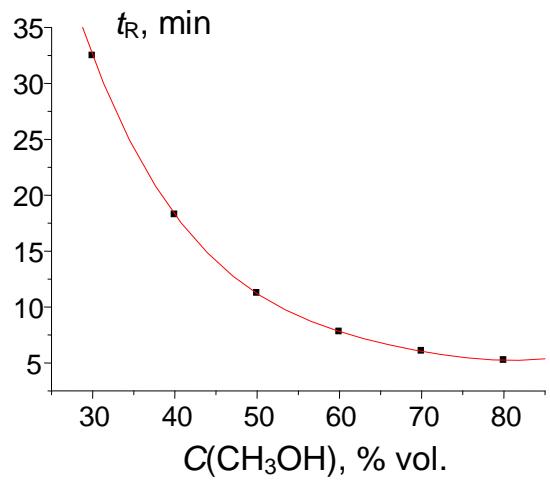 (a) 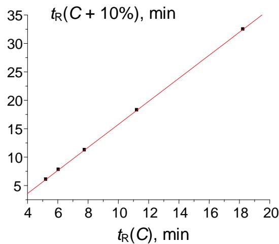 (b) Fig. 8: (a) Plot of the acetophenone retention time (min) vs. methanol concentration in the eluent, $t_{\mathrm{R}}(C)$: 32.464(30), 18.244(40), 11.230(50), 7.774(60), 6.052(70), and 5.226(80); (b) recurrent approximation of these data: $t_{\mathrm{R}}(C + 10\%) = at_{\mathrm{R}}(C) + b$. Parameters of the linear regression: $a = 0.4932 \pm 0.0005$, $b = 2.231 \pm 0.008$, $R = 0.99999$, $S_0 = 0.01$ (no outliers) Let us combine two theses. First, some organic compounds form hydrates and some of these hydrates are pretty stable. Several examples of such compounds are, for example: <table><tr><td>Compound</td><td>CAS no. of anhydrous form</td><td>CAS no. of hydrate</td></tr><tr><td>Glycine</td><td>56-40-6</td><td>130769-54-9</td></tr><tr><td>Oxalic acid</td><td>144-62-7</td><td>856335-90-5 (mono) 6153-56-6 (di)</td></tr><tr><td>Toluene</td><td>108-88-3</td><td>112270-21-0</td></tr><tr><td>Phenol</td><td>108-52-2</td><td>217182-78-0 144796-97-4</td></tr><tr><td>Nicotinamide</td><td>98-92-0</td><td>917925-73-6</td></tr><tr><td>Caffeine</td><td>58-08-2</td><td>5743-12-4</td></tr><tr><td>Methane (!)</td><td>74-82-8</td><td>14476-19-8</td></tr></table> CAS numbers obviously are different both for anhydrous and hydrated forms of the compounds mentioned. Such a number for a hydrate does not confirm its stability or isolation; it is the confirmation of interest in this hydrated form. It is interesting that this list even includes the simplest hydrocarbon, methane. Second, the separation of analytes in RP HPLC takes place in water-containing eluents, when the probability of hydrate formation is high. To identify the area in which anomalies should be expected, let us look again at Fig. 6. So far as the formation of hydrate of potassium acetate is most probable at low temperature of the aqueous solution, one anomalous leftmost point corresponds to the minimal values of solubility, $w(T)$. In HPLC eluents, the hydrate formation is most probable at the maximal water content of an eluent. Hence, the weird point in the $t_{\mathbb{R}}(C)$ plot should be located on the right. The plot in Fig. 9 represents the recurrent approximation of the set of retention times $t_{\mathbb{R}}(C)$ for 2-methoxybenzaldehyde oxime at retention times within the range of approx. 5-40 min. Four points belong to the single straight line with the correlation coefficient $R = 1.000$, but the rightmost point deviates downward from the regression line [10]. The formation of hydrates was confirmed experimentally for some oximes of aromatic carbonyl compounds [23, 24]. 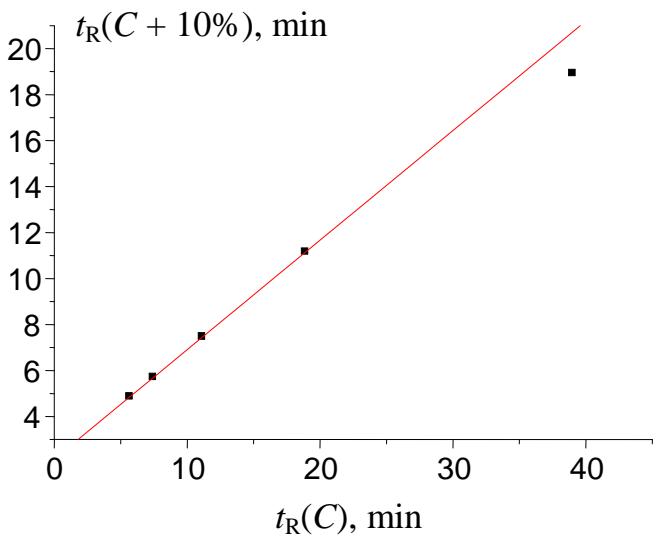 Fig. 9: The plot illustrating the anomaly (the rightmost point below the regression line) in the recurrent approximation of the retention times for 2-methoxybenzaldehyde oxime. Parameters of the linear regression (without outlier): $\mathbf{a} = 0.4763 \pm 0.0006$, $\mathbf{b} = 2.144 \pm 0.007$, $\mathbf{R} = 1.000$, $\mathbf{S}_0 = 0.006$. It is worth noting that deviations of the rightmost points in the plots of recurrent approximations of retention times in RP HPLC were detected for the first time for complex organic compounds, namely, synthetic antitumor sulfonamide drugs containing the polar functional group $-\mathrm{SO}_2$ -NRR' [9]. Most sulfonamides form stable hydrates, which can be isolated in a solid form [25-28]. Thus, the recurrent approximation of retention times in RP HPLC allows us to detect the reversible formation of hydrates of analytes. The possibility is all the more important considering that detecting hydrates using other methods is much more difficult. ## IV. CONCLUSION This manuscript provides a brief exploration of the applications of recurrent relations in chemistry and chromatography, acknowledging that it cannot encompass all possible examples. Nonetheless, the review highlights the significant potential of recurrent relations in simplifying calculations through the linearization of diverse chemical dependencies. The linearization achieved by recurrent relations not only streamlines mathematical manipulations but also reveals valuable insights from deviations in chemical dependencies. For instance, in reversed-phase high performance liquid chromatography (RP HPLC), non-linear variations in retention times can indicate hydration phenomena during analyte separation. Formally, two alternative conclusions emerge from our discussions. Firstly, a broad hypothesis posits that many monotonic chemical variables follow first-order recurrent dependencies — a potential general law in chemistry. However, a more modest yet preferable conclusion emphasizes the exceptional extrapolation capabilities of recurrent relations, which justify their widespread adoption in approximating a wide array of chemical variables. In conclusion, to make a reader smile, one humorous application of recurrences should be mentioned. There is a very nonlinear dependence of the time of drop falling of liquid (including wine) from an empty bottle, $t(n)$, on the serial number of the drop $(n)$. No idea concerning the analytical form of this function can be proposed (or, at least, it is rather difficult). However, the recurrent representation of this dependence, $t(n + 1) = at(n) + b$, demonstrates the excellent linearity [5].

Generating HTML Viewer...

References

27 Cites in Article
I Gutman,O Polanskii (1986). Mathematical Concepts in Organic Chemistry.
M Cockett,G Doggett (2012). Maths for Chemists. 2 nd Edn.
A Cunningham,R Whelan (2014). Math for Chemists.
Christopher Oriakhi (2021). Chemistry in Quantitative Language.
Igor Zenkevich (2009). Approximation of any physicochemical constants of homologues with the use of recurrect functions.
Igor Zenkevich (2009). Application of recurrent relationships in chromatography.
Igor Zenkevich (2010). Application of recurrent relations in chemistry.
I Zenkevich (2017). Recurrent Relationships in Separation Science.
Igor Zenkevich,Abdennour Derouiche,Darja Nikitina (2021). Detection of organic hydrates in reversed phase high performance liquid chromatography using recurrent approximation of their retention times.
Igor Zenkevich,Abdennour Derouiche (2024). Features and Advantages of the Recurrent Approximation of Retention Times in Reversed-Phase High-Performance Liquid Chromatography.
S Basin (1963). The Fibonacci Sequence As It Appears in Nature.
Parmanand Singh (1985). The so-called fibonacci numbers in ancient and medieval India.
T Brasch,J Bystrom,L Lystad (2012). Optimal control and the Fibonacci sequence.
D Lide,Ed (2003). CRC Handbook of Chemistry and Physics: A Ready-Reference of Chemical and Physical Data, 85th ed Edited by David R. Lide (National Institute of Standards and Technology). CRC Press LLC: Boca Raton, FL. 2004. 2712 pp. $139.99. ISBN 0-8493-0485-7..
Henry Henze,Charles Blair (1931). THE NUMBER OF ISOMERIC HYDROCARBONS OF THE METHANE SERIES.
H Henze,C Blair (1931). The number of structurally isomeric alcohols of the methanol series.
Douglass Perry (1932). THE NUMBER OF STRUCTURAL ISOMERS OF CERTAIN HOMOLOGS OF METHANE AND METHANOL.
J Song,R Thompson,T Vorburger,S Ballou,J Yen,T Renegar,A Zheng,R Silver,M Ols (2017). Establishing a Traceability and Quality System for U.S. Ballistics Identification Using NIST SRM Standard Bullets and Cartridge Cases.
E Soczewinski (1980). Quantitative retention-eluent composition relationships in liquid chromatography.
L Snyder,J Kirkland,J Dolan (2009). Introduction to modern liquid chromatography.
B Saifutdinov,V Davankov,M Il’in (2014). Thermodynamics of the sorption of 1,3,4-oxadiazole and 1,2,4,5-tetrazine derivatives from solutions on hypercrosslinked polystyrene.
B Saifutdinov,A Buryak (2019). The Influence of Water–Acetonitrile Solvent Composition on Thermodynamic Characteristics of Adsorption of Aromatic Heterocycles on Octadecyl-Bonded Silica Gels.
Bodil Jerslev,Sine Larsen,Emil Ratajczak,Alfred Sillesen,Julio Pellicer (1991). Hydrogen Bonding and Stereochemistry of Ring-Hydroxylated Aromatic Aldehyde Oximes. Crystal Structures of Three 4-OH-Substituted Benzaldehyde Oximes..
Bodil Jerslev,Sine Larsen,Antonio De La Hoz,Johan Springborg,Markku Sundberg,M Kady,S Christensen (1992). Crystallizations and Crystal Structure at 122 K of Anhydrous (E)-4-Hydroxybenzaldehyde Oxime..
P Suchetan,Sabine Foro,B Gowda,M Prakash (2012). 4-Chloro-<i>N</i>-(3-methylbenzoyl)benzenesulfonamide monohydrate.
A Kompella,S Kasa,V Balina,S Kusumba,B Adibhatla,P Muddasani (2024). Large scale Recurrent Relationships as an Important Class of Mathematical Equations in Chemistry Global Journal of Science Frontier Research ( B ).
No ethics committee approval was required for this article type.
Data Availability
Not applicable for this article.
How to Cite This Article
Igor G. Zenkevich. 2026. \u201cRecurrent Relationships as an Important Class of Mathematical Objects in Chemistry\u201d. Global Journal of Science Frontier Research - B: Chemistry GJSFR-B Volume 24 (GJSFR Volume 24 Issue B1): .
Explore published articles in an immersive Augmented Reality environment. Our platform converts research papers into interactive 3D books, allowing readers to view and interact with content using AR and VR compatible devices.
Your published article is automatically converted into a realistic 3D book. Flip through pages and read research papers in a more engaging and interactive format.
Recurrent relations combine the properties of arithmetic and geometric progressions, which accounts for their unique approximation abilities. This was illustrated by approximating the number of isomers of alkanes, the boiling points of homologs (nonlinear dependencies), the melting points of homologs (alternation effects), the temperature dependence of the solubility of inorganic salts in water, and by revealing the anomalies of gas chromatographic retention indices and retention times in reversed-phase high performance liquid chromatography.
Our website is actively being updated, and changes may occur frequently. Please clear your browser cache if needed. For feedback or error reporting, please email [email protected]
Thank you for connecting with us. We will respond to you shortly.