Response to Simply Supported Orthotropic Rectangular Plate Resting on a Variable Elastic Bi-Parametric Foundation under the Action of Moving Distributed Masses

Adeoye A.S; Adeloye T.O

I. INTRODUCTION

The problems connected with the analysis of thin structural bodies (rods, beams, plates, and shells) with other bodies have widespread application in various fields of science and technology. The physical phenomena involved in the impact event include structural responses, contact effects and wave propagation. These problems are topical issues of research in the field of applied mechanics. Since these problems belong to the problems of dynamic contact interaction, their solution is connected with severe mathematical and calculation difficulties. To this end, several researchers had worked and some are still working on the dynamic behavior of orthotropic rectangular plates. Analytical investigation of the low-velocity impact response of circular orthotropic and transversely isotropic plates possessing curvilinear anisotropy under compressive preloading has been carried out recently by Rossikhin and Shitikova in [1] and [2], respectively. The equations of plate motion take the rotatory inertia and transverse shear deformations into account. In the case of the orthotropic target [1], the changes in the geometrical dimensions of the contact domain have been ignored and the contact interaction is modeled by a linear spring, and a force arising in it is the linear approximation of Herts?z contact force. Ambartsumian [3] examined the five fundamental differential equations describing the equilibrium of an orthotropic plate with a cylindrical anisotropy for the case when all radial planes crossing the axis of anisotropy are the planes of elastic symmetry. Sveklo [4] suggested the contact theory for two anisotropic bodies under compression according to which the contact pressure is distributed over an elliptical contact region. The same structural effects are also true of the concrete slab in a composite girder bridge, but the steel orthotropic deck is considerably lighter, and therefore allows longer span bridges to be more efficiently designed. Awodola [5] studied the effect of plate parameters on the vibrations under moving masses of elastically supported plate resting on bi-parametric foundation with stiffness variation.Szekrenyes [6] investigated the interface fracture in orthotropic composite plates using second order shear deformation theory. Kadari [7] analyzed buckling in orthotropic nanoscale plates resting on elastic foundations. Yan [8] proposed elastic orthotropic models and used these in the nonlinear analysis of concrete structures subjected to monotonic or pseudo dynamic loading. Since these models can appropriately describe the strain softening behavior of concrete beyond the peak stress and show good agreement with the strength envelope obtained from experimental results Hu and Yao [9] studied the vibration solutions of rectangular orthotropic plates by symplectic geometry method. In the same vien, Alshaya, Hunt and Rowlands [10] investigated stresses and strains in thick perforated orthotropic plates. Gbadeyan and Dada [11] found the natural frequency of rectangular plates traversed by moving concentrated masses. Awodola and Adeoye [13] investigated the behavior of simply supported orthotropic rectangular plate by applying the technique of variable separable. Adeoye and Awodola [14] studied the dynamic behavior of orthotropic rectangular plate with clamped-clamped boundary conditions by making use of the technique of Shadnam Due to inability of researchers to solve orthotropic plates problems by analytical methods, this work aims at solving the governing equation by analytical solution and also considers the effect of the flexural rigidities in both x and y directions.

II. GOVERNING EQUATION

The dynamic transverse displacement $W(x,y,t)$ of orthotropic rectangular plates when it is resting on a bi-parametric elastic foundation and traversed by distributed mass $M_{r}$ moving with constant velocity $c_{r}$ along a straight line parallel to the x-axis issuing from point y=s on the y-axis with flexural rigidities $D_{x}$ and $D_{y}$ is governed by the fourth order partial differential equation given as

Ref

where $D_{x}$ and $D_{y}$ are the flexural rigidities of the plate along x and y axes respectively.

Notes

$E_{x}$ and $E_{y}$ are the Young's moduli along x and y axes respectively, $G_{o}$ is the rigidity modulus, $\nu_{x}$ and $\nu_{y}$ are Poisson's ratios for the material such that $E_{x}\nu_{y}=E_{y}\nu_{x}$ , $\rho$ is the mass density per unit volume of the plate, h is the plate thickness, t is the time, x and y are the spatial coordinates in x and y directions respectively, $R_{o}$ is the rotatory inertia correction factor, $K_{o}$ is the foundation constant, $S_{o}$ shear modulus and g is the acceleration due to gravity, H(.) is the Heaviside function.

Rewriting equation (2.1), one obtains

Simplifying equation (2.3) further, one obtains

III. ANALYTICAL APPROXIMATE SOLUTION

In order to solve equation (2.4), one applies technique of Shadnam et al which requires that the deflection of the plates be in series form as

where

The right hand side of equation (2.4), taken into account equation (3.1), written in the form of series takes the form

and zero when $n \neq m$

where

Making use of equation (3.3) and taking into account equation (3.2), equation (2.4) can be written as

Notes

On further simplification of equation (3.5), one obtains

The system of equations in equation (3.6) is a set of coupled ordinary differential equations where $H(x - c_{r}t)$ and $H(y - s)$ are the Heaviside functions which are defined as

With the properties

On putting equations (3.7) to (3.11) into equation (3.6) and simplifying, one obtains

Notes

$\Psi_{m}(x,y)$ is assumed to be the products of functions $\Psi_{pm}(x)\Psi_{bm}(y)$ which are the beam functions in the directions of x and y axes respectively. That is

Considering a unit mass, equation (3.12) can be re-written as

equation (3.42) is the fundamental equation of the problem. where

We shall consider the situation where the orthotropic rectangular plate is simply supported at all its edges. The boundary conditions for an orthotropic rectangular plate having simple supports at all its edges are given by

On putting equations (3.55) to (3.58) into equations (3.13) to (3.37), the integrals become

On solving equations (3.59) to (3.66),(3.72) and (3.78), and substituting into equation (47), one obtains

The solutions to equation $(3.84)$ shall be obtained by considering two cases:

a) Simply Supported Orthotropic Rectangular Plate Tranversed by Moving Force

For moving force problem, one sets $\varpi = 0$ in equation (3.84) which becomes

Notes

(3.85) On further simplification and re-arrangement, one obtains

where

Consider a parameter $\lambda * < 1$ for any arbitrary mass ratio $\lambda$ , defined as

It can be shown that

Retaining only $o(\lambda^{*})$ , one obtains

On putting equation (3.89) into equation (3.86), rewriting and simplifying further, one obtains

Expanding equation (3.91), and retaining only $o(\lambda^{*})$ , one obtains

Using Struble's technique, equation (3.92) can be rewritten as

Hence, the entire equation (3.92) becomes

Notes is the modified frequency for simply supported orthotropic rectangular plate traversed by moving force.

On solving equation (3.94) by Laplace transformation techniques one obtains

which on inversion becomes

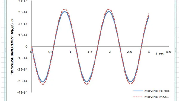
is the transverse displacement response to a moving force of a simply supported orthotropic rectangular plate.

b) Simply Supported Orthotropic Rectangular Plate Transversed by Moving Mass

Here, one seeks solution to the entire equation (3.84). To solve this problem, one makes use of the modified asymptotic method of Struble. The equation becomes,

On further simplifications and rearrangements of equation (3.98), one obtains

We shall consider a parameter $\alpha^{*} < 1$ for any arbitrary mass ratio defined by

On putting equation (3.101) into equation (3.99), expanding and retaining only $o(\alpha^{*2})$ , one obtains