Separability and a Lax Pair for the c_{2}{(1)} Toda lattice

Joachim Moussounda Mouanda; D. Dehainsala; G. F. Wankap Nono

I. INTRODUCTION
II. LINEARISATION OF TWO-DIMENSIONAL ALGEBRAIC COMPLETELY INTEGRABLE SYSTEMS
III. THE $C_2^{(1)}$ -TODA SYSTEM: ALGEBRAIC COMPLETELY INTEGRABILITY In this section, we recall some results relating the two-dimensional $\mathfrak{c}_2^{(1)}$ toda system. It is well known that this system is a.c.i. (see [12]).
1. Theorem 3.1. [12]
IV. SEPARATION OF THE VARIABLES
V. LAX PAIRS

I. INTRODUCTION

Completely integrable systems have been largely investigated during the past years. Some of them possess much richer structures that are the subject of extensive research and are called algebraic completely integrable system. This concept was introduced by Adler and van Moerbeke in [6]. An integrable polynomial system is algebraic completely integrable (a.c.i.) if the complexified system linearizes on an appropriate Abelian variety.

Many algebraic completely integrable systems possess matrix Lax representations whose spectral curves admit symmetries; in particular, involutions. The Jacobians of these curves contain Abelian subvarieties whose subsets are identified with the complex invariant manifolds of the system. The list of such systems includes the well known integrable cases of the Henon-Heiles systems [20], the integrable cases of quartic potentials [21], the Chaplygin top [8] and [14, 17], etc. A Lax representation for these systems can be constructed in terms of a direct product of Lax operators [20]. The literature on Lax equations is immense. The original references are [18, 15, 16, 4, 5]. Indeed, in order to simplify quantum problems it would be more convenient to use Lax representations in terms of $2 \times 2$ matrices.

In this paper, we consider the $\mathfrak{c}_2^{(1)}$ Toda lattice. It is a algebraic completely integrable (a.c.i.) system in the sense of Adler-van Moerbeke [2, 3] which means it can be linearized on a complex algebraic torus $\mathbb{C}^r / \wedge$ ( $\wedge$ a lattice in $\mathbb{C}^r$ ) i.e. an Abelian variety $\mathbb{T}^r$ . The aim is to find the separating variables and to show how to construct for this system a Lax representation. To this end, we use the algebraic structure of the problem. The separating variables give us a simple way of constructing a Lax equation. These separating variables can be found by inspecting the Painlevé expansions of the solutions near some special divisor on the compactified invariant manifolds of the problem.

In two dimensional, $\mathbb{T}^2$ is a Abelian surface. If $\mathbb{T}^2$ is Jacobian surface i.e. contains a smooth curve of genus two, then there exists a general procedure, due to Pol Vanhaecke [23] for finding the separating variables. It turns out, however, that the Abelian surface in the case of the $\mathfrak{c}_2^{(1)}$ Toda lattice is not a Jacobian surface [12]. Furthermore, if one of the components is a 2:1 unramified cover of a smooth curve of genus, the procedure still applies. We shall see this is the case for our two-dimensional a.c.i. system $\mathfrak{c}_2^{(1)}$ Toda lattice.

II. LINEARISATION OF TWO-DIMENSIONAL ALGEBRAIC COMPLETELY INTEGRABLE SYSTEMS

In this section, we recall some basic tools which will allow us to study algebraic completely integrable (a.c.i.) systems [6]. Consider the Hamiltonian system

where $H$ is the Hamiltonian and $J = J(x)$ is a skew-symmetric matrix with polynomial entries in $x$ , for which the corresponding Poisson bracket $\{H_i, H_j\} = \left\langle \frac{\partial H_i}{\partial x}, J \frac{\partial H_j}{\partial x} \right\rangle$ satisfies the Jacobi identity. The system (2.1) is integrable if it possesses $n + k$ independent polynomial invariants $H_1, \ldots, H_{n + k}$ of which $k$ invariants are Casimirs, the $n$ remaining ones are in involution and $m = 2n + k$ . The intersection

is invariant by Poisson-commutativity for the flows of all $\mathcal{X}_H$ , and is smooth for generic values of $c = (c_1, \ldots, c_m)$ . By the well-known Arnold-Liouville theorem, the compact connected components of these invariant manifolds are diffeomorphic to real tori. Moreover, the flows of vector field $\mathcal{X}_H$ are linear, when they are seen as flows on the tori using the diffeomorphism. The integer $n$ is called the dimension of the system.

The Poisson structure and the vector field are easily complexified, giving a Poisson-commuting family of functions on $\mathbb{C}^m$ and for generic $c = (c_1,\ldots,c_n)$ in $\mathbb{C}^{n + k}$ , the invariant manifolds

are smooth affine (algebraic) varieties. In this case, the integrable system will be called algebraic completely integrable if these generic invariant manifolds $\mathcal{A}_c$ are smooth affine parts of an Abelian variety $\mathbb{T}_c^n$ and the flows of integrable vector fields are linear. This means that $\mathcal{A}_c = \mathbb{T}_c^n\setminus \mathcal{D}_c$ , where $\mathcal{D}_c$ is the minimal divisor with the coordinate functions $x(t)$ , restricted to the invariant manifolds, blow up for some value of $t\in \mathbb{C}$ and if the (complex) flow of the vector fields on $\mathbb{T}_c$ is linear [23].

In the two-dimensional case, that is $n = 2$ , the invariant manifolds complete into Abelian surfaces by adding one (or several) curves to the affine surfaces $\mathcal{A}_c$ . In this case, Vanhaecke proposed in [23] a method which leads to an explicit linearization of the vector field of the a.c.i. system. The computation of the first few terms of the Laurent solutions to the differential equations enables us to construct an embedding of the invariant manifolds in the projective space $\mathbb{P}^N$ . From this embedding, one deduces the structure of the divisors $\mathcal{D}_c$ to be adjoined to the generic affine $\mathcal{A}_c$ in order to complete them into Abelian surfaces $\mathbb{T}_c$ . Thus, the system is a.c.i.. The different steps of the algorithm of Vanhaecke are given by:

(a) If one of the components of $\mathcal{D}_c$ is a smooth curve $\Gamma_c$ of genus two, compute the image of the rational map $\phi_{[2\Gamma_c]}:\mathbb{T}_c^2\to \mathbb{P}^3$ which is a singular surface in $\mathbb{P}^3$ , the Kummer surface $\mathcal{K}_c$ of the jacobian $\operatorname {Jac}(\Gamma_c)$ of the curve $\Gamma_c$ .

(b) Otherwise, if one of the components of $\mathcal{D}_c$ is a $d:1$ unramified cover $\mathcal{C}_c$ of a smooth curve $\Gamma_c$ of genus two, the map $p:\mathcal{C}_c\to \Gamma_c$ extends to the map $\widetilde{p}:\mathbb{T}_c^2\to \mathrm{Jac}(\Gamma_c)$ . In this case, let $\mathcal{C}_c$ denote the (non complete) linear system $\widetilde{p}^{*}[2\Gamma_{c}]\subset [2\mathcal{C}_{c}]$ which corresponds to the complete linear system $[2\mathcal{C}_c]$ and compute now the Kummer surface $\mathcal{C}_c$ of $\operatorname {Jac}(\Gamma_c)$ as image of $\phi_{\mathcal{E}_c}:\mathbb{T}_c^2\to \mathbb{P}^3$ .

(c) Otherwise, change the divisor at infinity so as to arrive in $\operatorname{cas}(a)$ or $(b)$ . This can always be done for any irreducible Abelian surface.

Choose a Weierstrass point $W$ on the curve $\Gamma_c$ and coordinates $(z_0: z_1: z_2: z_3)$ for $\mathbb{P}^3$ such $\phi_{[2\Gamma_c]}(W) = (0: 0: 0: 1)$ in case 1.(a) and $\phi_{\mathcal{E}_c}(W) = (0: 0: 0: 1)$ in case 1.(b). Then this point will be a singular point (node) for the Kummer surface $\mathcal{K}_c$ whose equation is

where the $p_i$ are polynomials of degree $i$ . After a projective transformation which fixes $(0:0:0:1)$ , we may assume that $p_2(z_o, z_1, z_2) = z_1^2 - 4z_0z_2$ .

Finally, let $x_{1}$ and $x_{2}$ be the roots of the quadratic equation $z_{0}x^{2} + z_{1}x + z_{2} = 0$ , whose discriminant is $p_{2}(z_{o},z_{1},z_{2})$ , with the $z_{i}$ expressed in terms of the original variables. Then the differential equations describing the vector field of the system are rewritten by direct computation in the classical Weierstrass form

where $\alpha_{1}$ and $\alpha_{2}$ depend on $c$ (i.e., on the torus). From it, the symmetric functions $x_{1} + x_{2} (= -z_{1} / z_{0})$ , $x_{1}x_{2} (= z_{2} / z_{0})$ and the original variables can be written in terms of the Riemann theta function associated to the curve $y^{2} = f(x)$ .

III. THE $C_2^{(1)}$ -TODA SYSTEM: ALGEBRAIC COMPLETELY INTEGRABILITY In this section, we recall some results relating the two-dimensional $\mathfrak{c}_2^{(1)}$ toda system. It is well known that this system is a.c.i. (see [12]).

The Toda lattice associated to the twisted affine Lie algebra $\mathfrak{c}_2^{(1)}$ consists of three particles interconnected by means of exponential springs and constrained to move on a circle. The motion is determined by the following equations

on the hyperplane $\mathcal{H} = \left\{(x_0, x_1, \ldots, x_5) \in \mathbb{C}^6 \mid x_3 + 2x_4 + x_5 = 0\right\}$ . We denote by $\mathcal{V}$ the vector field defined by the above differential equations(3.1).

There are three independent constants of motion, namely

The field $\mathcal{V}$ is the Hamiltonian vector field with the function $F_{2}$ , with respect to the Poisson structure defined by the following skew-symmetric matrix

If we assign $x_0, x_1$ and $x_2$ weight 2 and $x_3, x_4$ and $x_5$ weight 1, then the invariants are all homogeneous with weights 8, 2 and 4 respectively. If we give time weight $-1$ , the vector field $\mathcal{V}$ also becomes weight homogeneous. It is shown in [6] that, for such vector field, it is easy to find the weight homogeneous Laurent solutions to the differential equations. On $\mathbb{C}^6$ there are two involutions $\sigma$ and $\tau$ which preserve the constants of motion $F_1, F_2$ and $F_3$ . These involutions, restrict to the hyperplane $\mathcal{H}$ , are given by

The involution $\sigma$ preserves the vector field $\mathcal{V}$ (3.1) while the involution $\tau$ changes its sign. Both involutions will have strong implications on the geometry of the integrable system [12]. We have shown [12] that the set of regular values of the momentum map $\mathbb{F}$ is the Zariski open in $\mathbb{C}^3$ given by

Throughout the rest, a generic point $c = (c_{1}, c_{2}, c_{3})$ in $\mathbb{C}^3$ will be an element of the set $\Omega$ .

The involution $\sigma$ simplifies the Painlevé analysis to the system. We show that the system of differential equations (3.1) possesses three families of Laurent solutions depending on the maximal number free parameters (4 in this case). Such families are called principal balances. The first principal balance $x(t, m_0)$ is given by

where the four free parameters have been denoted by $a, c, d$ and $e$ . The second principal balance $x(t; m_1)$ is given by

where the four free parameters are denoted by $\alpha, \beta, \gamma$ and $\delta$ . The last principal balance $x(t; m_2)$ is obtained from the above formulas for $x(t; m_0)$ by applying the involution $\sigma$ . Using the majorant method[6], one shows that these series are convergent for small $|t| \neq 0$ .

Substituting the Laurent solution (3.6) into (3.2): $F_{1} = c_{1}$ , $F_{2} = c_{2}$ and $F_{3} = c_{3}$ , and equaling the $t^0$ -terms yields $c_{1} = 4ce^{2}$ , $c_{2} = a^{2} - 4c - 12d$ , $c_{3} = 48cd - 12a^{2}d - 32ae$ . Eliminating $c$ and $d$ from these equations leads to an equation connecting the two remaining parameters $a$ and $e$ . Namely,

It is shown in [9, 12] that this curve can be compactified into a Riemann surface, denoted by $\overline{\Gamma}_c^0$ , by just adding six points at infinity and the genus of $\overline{\Gamma}_c^0$ is two. Upon computing the abstract Painlevé divisor $\Gamma_c^2$ , which corresponds to the Laurent solution $x(t,m_2)$ , we obtain the same equation (3.8), since the involution $\sigma$ preserves the constants of motion, so that the Riemann surface $\overline{\Gamma}_c^2$ is isomorphic to $\overline{\Gamma}_c^0$ .

At last, a direct substitution of the Laurent solution $x(t; m_1)$ (3.7) in the three equations $F_i = c_i$ , $i = 1,2,3$ ; leads to the algebraic equations in terms of the four parameters $\alpha, \beta, \gamma$ and $\delta$ , to wit

Since $c_{1} \neq 0$ , by eliminating the parameters $\gamma$ and $\delta$ in these equations, we find a curve $\Gamma_c^1$ whose equation is given, in the two remaining parameters $\alpha$ and $\beta$ , by

For $c$ generic, the affine curve $\Gamma_c^1$ is smooth and can be compactified into a Riemann surface, denoted $\overline{\Gamma}_c^1$ , by adding two points at infinity $\infty'$ and $\infty''$ . A local parametrization of neighborhood of these points is given by

The genus of the Riemann surface $\overline{\Gamma}_c^1$ is three. Indeed, by making the change of the variable $\xi = 128\beta + (4c_3 - (4\alpha^2 - c_2)^2)$ , we can see that the curve $\overline{\Gamma}_c^1$ is isomorphic to the smooth genus three hyperelliptic Riemann surface $\mathcal{C}_c^1: \xi^2 = h(\alpha) = ((4\alpha^2 - c_2)^2 - 4c_3)^2 - 16384c_1$ .

The affine invariant surface

defined by the three constants of motion can be embedded in the projective space $\mathbb{P}^{17}$ means of eighteen functions

z _ {1 5} = x _ {1} x _ {0} igl(4 x _ {1} igl(x _ {3} - 2 x _ {5}igr) + x _ {5} igl(x _ {5} ^ {2} - 4 x _ {2}igr)igr),

which behave like $t^{-1}$ at worst when the three principal balances are substituted into them. Using the embedding

and the three principal balances, it is possible to show that the closure of the image of this affine surface $\mathbb{F}_c$ is an Abelian surface $\mathbb{T}_c^2$ for generic values $c = (c_1,c_2,c_3)\in \Omega$ of constants of motion. Indeed, the map $\varphi_{c}$ induces three injective maps $\varphi_c^i:\Gamma_c^i\to \mathbb{P}^{17}$ $(i = 0,1,2)$ that define the divisor $\mathcal{D}_c$ to be added to $\mathbb{F}_c$ for its completion into the Abelian surface $\mathbb{T}_c^2$ . The closure of the image of each of these maps, $\overline{\varphi_c^i(\Gamma_c^i)}$ will be denoted by $\mathcal{D}_c^i$ . We have the following result:

Theorem 3.1. [12]

For generic points of $\mathbb{C}^3$ , the invariant surface $\mathbb{F}_c$ is the affine part of an Abelian surface $\mathbb{T}_c^2$ . The divisor at infinity $\mathcal{D}_c$ on $\mathbb{T}_c^2$ consists of three irreducible components $\mathcal{D}_c^0$ , $\mathcal{D}_c^1$ and $\mathcal{D}_c^2$ where (a) $\mathcal{D}_c^0$ and $\mathcal{D}_c^2$ are both singular curves isomorphic to $\overline{\Gamma}_c^0$ defined by

(b) $\mathcal{D}_c^1$ is isomorphic to the smooth hyperelliptic curve of genus three $\overline{\Gamma}_c^1$ defined by

The system of differential equations (3.1) is algebraically completely integrable and the flows of integrable vector fields are linear on the Abelian surfaces $\mathbb{T}_c^2$ .

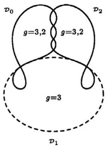
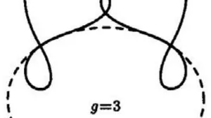
Remark 3.2. The divisor that completes the invariant surface $\mathbb{F}_c$ into Abelian surface is made up by three curves $\mathcal{D}_i\coloneqq \mathcal{D}_c^i$ . $\mathcal{D}_1$ intersects the over curves at one point each. The letter intersect each other at four points.

IV. SEPARATION OF THE VARIABLES

This section is entirely devoted to the linearization of the system. As we have seen in the previous section, a two-dimensional algebraic completely integrable system is linearizable if one of the components of the divisor $\mathcal{D}_c$ (to be adjoined to $\mathbb{F}_c$ in order to complete $\mathbb{F}_c$ into an Abelian surface) is a smooth curve of genus two; which is not the case for our system. Indeed, $\mathbb{T}_c^2$ is not a Jacobian surface because one of the components of $\mathcal{D}_c$ is not a smooth curve of genus two. We show in [12] that $\mathbb{T}_c^2$ is Prym variety of polarization of type $(1,2)$ . In this situation, according to Vanhaecke, the system is linearizable if one of the components of $\mathcal{D}_c$ is a $d:1$ unramified $\mathcal{C}_c$ of a smooth curve of genus two. In order to check this condition, we consider the curve $\overline{\Gamma}_c^1$ defined by

which is a component of the divisor $\mathcal{D}_c$ . For $c \in \Omega$ , the curve $\overline{\Gamma}_c^1$ is a smooth hyperelliptic curve of genus three. The involution $\sigma: (x_0, x_1, x_2, x_3, x_4, x_5) \mapsto (x_2, x_1, x_0, x_5, x_4, x_3)$ acts on the parameters $\alpha, \beta, \gamma$ and $\delta$ in the following way:

For generic $c$ , $\beta \delta = c_{1} \neq 0$ . It follows that the map

is an involution for the curve $\overline{\Gamma}_c^1$ . Indeed, let $\sigma$ be the involution which acts on the curve $\overline{\Gamma}_c^1$ , the equation (4.1) becomes

Simplifying by $\frac{c_1}{\beta}$ , this leads to

which can be written as

Since $\beta \neq 0$ , we find the same initial equation of the curve $\Gamma_c^1$ . Namely,

Remark 4.1. The invariants of the involution $\sigma$ are

Indeed, we have $\sigma(Z) = -\alpha\left(\frac{c_1}{\beta} - \beta\right) = \alpha\left(\beta - \frac{c_1}{\beta}\right) = Z$ ; clearly we have $\sigma(Y) = Y$ and $\sigma(X) = X$ .

Proposition 4.2. Let $\mathcal{K}_c$ be the quotient of the curve $\overline{\Gamma}_c^1$ by the involution $\sigma$ . For generic $c$ , the quotient curve $\mathcal{K}_c$ is a smooth curve of genus two and the map $\overline{\Gamma}_c^1 \to \mathcal{K}_c$ is an unramified $2:1$ map.

Proof. We determine the genus of the curve $\mathcal{K}_c\coloneqq \overline{\Gamma}_c^1 /\sigma$ . We observe that the equation of $\overline{\Gamma}_c^1$ can be written in the following form:

such that

We deduce that

On the other hand, we have

Substituting (4.4) in (4.5), one obtains the equation of the curve $\mathcal{K}_c$ . Namely

Thus, the curve $\mathcal{K}_c$ is isomorphic to the hyperelliptic of genus two whose the equation is

For $c \in \Omega$ , this curve is smooth because the polynomial $h(y)$ is without multiple roots; indeed, its discriminant is equals, up to a constant, to

which does not vanish for $c \in \Omega$ . Finally let us show that the involution $\sigma$ has no fixed point for $c \in \Omega$ . A point $(x_0, x_1, x_2, x_3, x_4, x_5)$ de $\mathbb{F}_c$ is a fixed point for involution $\sigma$ if and only if $x_0 = x_2$ and $x_3 = x_5$ . By substituting the coordinates $x_2$ and $x_5$ respectively by $x_0$ and $x_3$ in the functions $F_i = c_i$ (for $i = 1,2,3$ ), one obtains the system

By a direct computation, we find the relation $c_2^2 - 4c_3 = 128x_0x_1$ . This leads to the equality

which is impossible for a generic point $c \in \mathbb{C}^3$ . Thus the involution $\sigma$ has no fixed point in $\mathbb{F}_c$ . Using (4.2), it is easy to verify that the points at infinity $\infty'$ and $\infty''$ also aren't fixed points for $\sigma$ . We have

We can conclude that the map $\pi: \overline{\Gamma}_c^1 \longrightarrow \mathcal{K}_c$ is an unramified double cover.

Theorem 4.3. The vector field $\mathcal{V}$ (3.1) extends to a linear vector field on the Abelian surface $\mathbb{T}_c^2$ and the Jacobi form for the differentials equation can be written as

where $f(\mu) = \left(\mu^4 - 2c_3\mu^2 - 1024c_1 + c_3^2\right)\left(\mu - \frac{1}{2}c_2\right)$ ; and the curve $v^2 = f(\mu)$ is birational equivalent to the hyperelliptic curve of genus two $\mathcal{K}_c$ (4.6).

Proof. The demonstration is based on the Vanhaecke's procedure described above. We first construct, following [7], an explicit map from the generic fiber $\mathbb{F}_c$ into the Jacobian of the Riemann surface $\overline{\Gamma}_c^1$ .

We consider the functions which have at worst a double pole along the component $\mathcal{D}_c^1$ of the divisor $\mathcal{D}_c$ on $\mathrm{Jac}(\overline{\Gamma}_c^1)$ , and no others poles. These functions are obtained by constructing those polynomials on $\mathcal{H}$ which have at worst a double pole in $t$ when the principal balance $x(t,m_1)$ is substituted into them and no poles when the other principal balances are substituted.

From (3.7), we easily show that the space of such polynomials is spanned by

The leading terms are given by

Among these functions, only the following are invariants by the involution $\sigma$ :

The above functions allow us to embed the Kummer surface of $\operatorname{Jac}(\mathcal{K}_c)$ in the projective space $\mathbb{P}^3$ . Consider now the Koidara map which correspond to these functions.

Since the functions $\theta_{i}$ correspond to the sections of the line bundle $\left[2\mathcal{D}_c^1\right]$ , the map $\varphi_c$ maps the $\operatorname{Jac}(\mathcal{K}_c)$ into its Kummer surface, which is a singular quartic in the projective space $\mathbb{P}^3$ .

An equation for this quartic surface, in terms of $\theta_{i}$ , can be computed by eliminating the variables $x_0, x_1, x_2, x_3, x_5$ from (4.7) and from the equations

The result is a quartic equation of the Kummer surface of $\operatorname{Jac}(\mathcal{K}_c)$ which it can be put in the following form:

where $P_{3}$ (respectively $P_{4}$ ) is a polynomial of degree three (respectively four) in $\theta_{1}$ and $\theta_{2}$ , given by

The coefficient of $\theta_{3}$ in (4.10) can be written, in terms of the initial variables $x_0,x_1,x_2,x_3$ and $x_{5}$ , as follows:

Let $\mu_{1}$ and $\mu_{2}$ be roots of the polynomial

By [23, Theorem 9], the vector field $\mathcal{V}$ defining the Toda lattice linearizes upon the setting

which implies, with respect to the vector field $\mathcal{V}$ , that

Substituting (4.11) and (4.12) in the invariants (4.9) and eliminating the variables $x_0, x_1, x_2, x_3$ and $x_5$ , two quadratic polynomials in $\dot{\mu}_1^2$ and $\dot{\mu}_2^2$ are found. Solving them for in $\dot{\mu}_1^2$ and $\dot{\mu}_2^2$ yields

It follows that

where $f$ is the polynomial

Integrating (4.13) we see that the field $\mathcal{V}$ is a linear vector field on $\mathbb{F}_c$ which obviously extends to linear vector field on the Jacobian variety of the curve $\kappa_{c}$ and the factor of its generic complex invariant manifold $\mathbb{F}_c$ by $\sigma$ is an open subset of $\operatorname {Jac}(\mathcal{K}_c)$ .

By using [19, Theorem 5.3], we show that the symmetric functions $\mu_{1}$ , $\mu_{2}$ and the original phase variables can be written in terms of theta functions.

In this connection, a natural question is how the curve $\mathcal{K}_c$ and the curve $v^2 = f(\mu)$ are related. The answer comes out immediately when we observe that the curves $v^2 = f(\mu)$ and $\mathcal{K}_c$ are birationally equivalent. Indeed, setting $u = \mu - c_2 / 2$ , we obtain the following:

Next, putting $y = -2u$ , and $z = 4i\sqrt{2} v$ , we obtain the equation

of the curve $\mathcal{K}_c$ whose the jacobian is canonically associated to the Abelian surface $\mathbb{T}_c^2$ .

V. LAX PAIRS

In this Section, we shall find a new Lax pair for the $c_2^{(1)}$ Toda lattice.

Let $u, v$ and $w$ be functions in $t$ with the property $uw + v^2 = c$ , $c$ is a constant. Then the following obvious identity holds

where

Suppose that a completely integrable Hamiltonian system is given which linearizes on a Jacobian variety $\operatorname{Jac}(\Gamma)$ of a hyperelliptic curve $\Gamma: y^2 = f(\lambda)$ , where $f(\lambda)$ is a polynomial with coefficients depending upon the constant of motion. Then, as it has been first by Fairbanks [13] and also Pol Vanhaecke [23], we may take $c = f(\lambda)$ , and define $u, v, w$ to be the Jacobi polynomials on $\operatorname{Jac}(\Gamma)$ . Thus we obtain a Lax pair (5.1) depending on a spectral parameter $\lambda$ , and the coefficients of $f(\lambda)$ (and hence the first integrals) are reconstructed from the identities

Suppose first that the curve $\Gamma$ is a genus 2 curve. Let $p_1$ and $p_2$ be points on $\Gamma$ and denote $\mu_1 = \lambda(p_1)$ , $\mu_2 = \lambda(p_2)$ . Then the Jacobi polynomials associated with $\Gamma$ read

Note that $w(\lambda)$ is in fact a polynomial in $\lambda$ .

Let us find now a new Lax pair for the $c_{2}^{(1)}$ Toda lattice. According to Mumford's description of hyperelliptic Jacobians (see [19, Section 3.1]), if $\Gamma$ a hyperelliptic curve of genus two then the Riemann surface $\overline{\Gamma}$ is embedded in its jacobian in a such way that $\operatorname{Jac}(\overline{\Gamma}) \setminus \Gamma$ is isomorphic to the space of pairs of polynomials $(u(\lambda), v(\lambda))$ such that $u(\lambda)$ is a monic of degree two, $v(\lambda)$ is of degree less than two and $f(\lambda) - v^{2}(\lambda)$ is divisible by $u(\lambda)$ . Let us describe the map from $\mathbb{F}_c$ into $\operatorname{Jac}(\overline{\Gamma}_c^1)$ in terms of these polynomials. Let $\mu_1$ and $\mu_2$ be the roots of the polynomial $u(\lambda)$ . From (4.11), we can conclude that

The polynomial $v(\lambda)$ is defined as the derivative, suitable normalised, of $u(\lambda)$ in the direction of the vector field $\mathcal{V}$ (3.1), we find out that

It is easy to check that the expression $f(\lambda) - v^2 (\lambda)$ is divisible by $u(\lambda)$ such that the above formulas define a point of $\operatorname {Jac}(\overline{\Gamma}_c^1)\setminus \Gamma_c^1$ . Let's put

$w(\lambda)$ is a polynomial in $\lambda$ of degree $3 = \deg u + 1$ . By direct calculation, we find

where

and

Based on above and [22, Chapter VII.2], the linearizing variables (4.11) and (4.12) suggest a morphism $\phi$ from the $\mathfrak{c}_2^{(1)}$ Toda lattice to genus 2 odd Mumford system:

It is well known that the Mumford system $\mathcal{M}$ is algebraic completely integrable. The morphism $\phi: \mathcal{H} \to \mathbb{C}^7$ is given by

The form of the Lax pair then follows from [23]. We have:

Theorem 5.1. The Lax equation for the Hamiltonian vector field $\mathcal{V}$ is given by

by taking

where $u(\lambda), v(\lambda)$ and $w(\lambda)$ are the polynomials defined above. The coefficient $b(\lambda)$ of the matrix $Y(\lambda)$ is the polynomial part of the rational function $w(\lambda) / u(\lambda)$ .

By direct computation, one finds

And we can show that the characteristic polynomial of the matrix $X(\lambda)$ is precisely the polynomial which defines the curve $\mathcal{K}_c$ .

We grateful to Pol Vanhaecke for stimulating discussions and suggestions we had together on this paper. We wish to express our thanks to an anonymous referee for his valuable helpful comments and suggestions

[1] Adler, M., van Moerbeke, P., The Kowalewski and Hénon-Heiles motions as Manakov geodesic flows on $SO(4)$ : a two-dimensional family of Lax pairs. Comm. Math. Phys., 1988, vol. 113, no. 4, pp. 659-700.
[2] Adler, M. and van Moerbeke, P., The algebraic integrability of geodesic flow on SO(4). Invent. Math., 1982, vol. 67, no. 2, pp. 297-331.
[3] Adler, M. and van Moerbeke, P., The complex geometry of Kowalevski-Painlev analysis. Invent. Math., 97 (1989), pp. 3-51.
[4] Adler, M. and van Moerbeke, P., Completely integrable systems, Euclidean Lie algebras, and curves. Adv. Math., 38 (1980), pp. 267-317.
[5] Adler, M. and van Moerbeke, P., Linearization of Hamiltonian systems, Jacobi varieties and representation theory. Adv. Math., 38 (1980), pp. 318-379.
[6] Adler, M. and van Moerbeke, P. and Vanhaecke, P., Algebraic integrability, Painlevé geometry and Lie algebras. Ergeb. Math. Grenzgeb. (3), vol. 47, Berlin-Heidelberg: Springer, 2004.
[7] Bueken, P., and Vanhaecke, P., The moduli problem for integrable systems: the example of a geodesic flow on $SO(4)$ . J. London Math. Soc. (2), 62 (2), pp. 357-369, 2000.
[8] Chaplygin, C. A., New case of rotation of rigid body with a fixed point. Gostekhizdat, Moscow, 1954, pp. 472-476.
[9] Dehainsala, D., Sur l'intégrabilité algébrique des réseaux de Toda: cas particuliers des rseaux $\mathfrak{c}_2^{(1)}$ et $\mathfrak{d}_3^{(2)}$ . PhD thesis, University of Poitiers, 2008.
[10] Dehainsala, D., Sur l'intégrabilité algébrique des réseaux de Touta $\mathfrak{d}_3^{(2)}$ . C. R. Acad. Sci. Paris, Ser. I 437 (2009).
[11] Dehainsala, D., Algebraic integrability and geometry of the $\mathfrak{d}_3^{(2)}$ Toda lattice. Regular and Chaotic Dynamics, 2011, Vol. 16, Nos. 3-4, pp. 330-355.
[12] Dehainsala, D., Algebraic completely integrability of the $\mathfrak{c}_2^{(1)}$ Toda lattice, Journal of Geometry and Physics, 135 (2019), pp. 80-97.
[13] Fairbanks, L., Lax equations representation of certain completely integrable systems. Comp. Math., 1988, Vol. 68, No. 1, pp. 31-40.
[14] Fernandes, R. L., Vanhaecke, P., Hyperelliptic Prym varieties and integrable systems. Comm. Maths. Phys., 221(1) (2001), pp. 169-196.
[15] Flaschka, H., Toda Lattice I. Existence of Integrals. Phys. Rev. B., 9 (1980), pp. 1924-1925.
[16] Flaschka, H., Toda Lattice II. Inverse scattering evolution, Progr. Theoret. Phys., 51 (1974), pp. 703-716.
[17] Inoue, R., Vanhaecke, P., Yamazaki, T., The algebraic integrable systems related to spectral curves with automorphisms. J. Geom. Phys., 87 (2015), pp. 198-216.
[18] Lax, P., Integrals of nonlinear evolution equations and solitary waves. Comm. Pure Appl. Math., 21 (1968), pp. 467-490.
[19] Mumford, D., Tata lectures on theta.

II. Progress in Mathematics, Birkhäuser Boston Inc., 1984, Vol. 43.

[20] Ravoson, V., Gravilov, L., Gaboz, R., Separability and Lax pair for Hnon-Heiles system. J. Maths. Phys., 193, 34(6): 2385-2390.
[21] Ravoson, V., Ramani, A., Gramaticos, B., Generalized separability for a Hamiltonian with nonseparable quartic potential. Phys. Lett, 1994, Vol. 191, pp. 91-95.
[22] Vanhaecke, P., Integrable systems in the realm of algebraic geometry. 2nd ed., Lecture Notes in Math., vol. 1638, Berlin: Springer, 2001.
[23] Vanhaecke, P., Linearising two-dimensional integrable systems and the construction of action-angle variables. Math. Z., 1992, vol. 211, no. 2, pp. 265-313.