## I. INTRODUCTION Since the middle of the twentieth century, the quantitative landscape for modelling the performance of financial asset allocation has been pictured. Concretely, an investor would like to buy or sell some shares of a portfolio constituted of equities, commodities, cryptos, or derivatives, and wishes to allocate efficiently and with risk control. Markowitz is considered to be the first to have introduced a quantitative theory for allocating assets in an optimized manner, for a given targetted portfolio return [Markowitz]. For such portfolios, performance is measured in terms of portfolio return, while a common metric for risk is its standard deviation. Different metrics are used to measure performance of the portfolio [Sharpe, Riposo]. From this framework, many other quantitative approaches have been developed (see for example [Grinold, Cartea, Brugière]), all aiming at bringing profit to a risky investor. Generally speaking, a paradigm consists in expressing the portfolio return $R$ (vector of real numbers) as follows: $$ R = r _ {0} + \beta \left(R _ {\mathrm {M}} - r _ {0}\right) + \epsilon , \tag {1} $$ where $r_0$ is the return of a risk-free asset (for instance a bond) considered in the portfolio economy, $R_{\mathrm{M}}$ is the market return, $\beta$ is the exposure of the market to the investment portfolio, and $\epsilon$ is all the information not considered in the first and second terms of this equation. This equation can be proven through the Capital Asset Pricing Model (CAPM) (one of the main building-block articles for the CAPM is [French], and it was introduced by J. Treynor, W.F. Sharpe, J. Lintner, and J. Mossin, independently). In particular, the quantity $R_{\mathrm{M}} - r_0$ is the risk premium [Capinski]. However, the Markowitz framework may not be the best one to explain the risk taken by the investor to elaborate her portfolio, as risks are not specifically identified. In order to address risk dependencies, factor models have been introduced (for instance [Brugière, Connor]). If the returns are $R$, a general factor model writes as: $$ R = A + B F + \mathcal {E}. \tag {2} $$ where $A$ is a constant vector, $B$ is the matrix (number of assets × number of factors) of factor exposures, $F$ is the vector (dimension is the number of factors) of factor characteristics, and $\mathcal{E}$ is the vector gathering all the information which is not in the first two terms of the above equation. Generally speaking, the factor exposures represent the covariance of the returns with respect to the factor characteristics, and essentially represent how strongly dependent are the returns on the underlying factors (see [Klephish] for a conciliating estimation of risk factor exposures). The factor characteristics are of two types. (i) Endogeneous: they are statistically derived from the observed returns [FrenchR]; and (ii) Exogeneous: they are explanatory variables added to the model, for instance Growth, Price-to-Earning, Price-to-Book, or other fundamental metrics. In the sequence of this paper, we shall focus on the second type of factor characteristics. As an example of such characteristic portfolios, the Fama and French Three Factor Model [Fama] still has some strong supporters today. However, in the recent decades, most researchers have shown the existence of factor risk premium associated with specific factors as Value, Momentum, Size, Low Volatility, and Quality, see e.g. [Fitzgibbons, Bender, Ghayur]. Many discussions are redefining some factors as actually reflecting one of these five core factors, see e.g. [FrenchR2]. We will not enter the financial context of these five factors, the interested reader can focus on [Zaher]. Earlier studies in the style factors have seen researchers use a long-short approach aiming to capture the pure premium. Much inspired by Markowitz's, optimised portfolios have then been widely used in constructing factor portfolios. Optimization has the flexibility of introducing extra construction considerations simply as constraints without compromising ex-ante objective, providing the problem remains feasible and solvable, e.g. convex [Wilhelm]. Another construction method that has been introduced since the early days of portfolio construction is Tilting. Assets under management mostly using Tilting reached $1.45 trillion in December 2021 [Morningstar]. The Target Exposure framework, first introduced to the passive investment community by FTSE Russell indices, is an extension of traditional tilting and which has many practical use cases, e.g. [Wang]. The motivation was to join the transparency and intuition of tilting with the ability to exert explicit control of the portfolio ex-ante outcome that is comparable to optimisation. In short, and as shown in Section 2, the Target Exposure methodology aims at solving a system of exponential functions, giving at final a portfolio allocation (see Equation (6)). In this paper, we are not going to compare different approaches, as this is out of scope, and this will be interesting areas for further studies. We are focusing on the roots (or solutions) of a non-linear system of equations, the detailed form of which will be discussed in Section 2. In essence, the system of interest writes as: $$ \left\{ \begin{array}{l l} \mathcal {F} _ {1} (\alpha_ {1}, \ldots , \alpha_ {F}) & = 0 \\ \mathcal {F} _ {2} (\alpha_ {1}, \ldots , \alpha_ {F}) & = 0 \\ & \vdots \\ \mathcal {F} _ {F} (\alpha_ {1}, \ldots , \alpha_ {F ^ {\prime}}) & = 0 \end{array} \right. $$ where the $\mathcal{F}_f$ 's, $f \in \{1,2,\ldots,F\}$, are sums of product of exponential functions, see Equations (6). We want to check rather if there exists common root(s) for all the $\mathcal{F}_f$, $f \in \{1,2,\ldots,F\}$. Many methods have already been developed to solve such non-linear systems, by means of Taylor's polynomial [Burden], quadrature formula [Darvishi, Babajee], or homotopy perturbation method [Golbabai]. A gradient decent method could also be applied to solve such system [Hao]. Using more contemporary approaches, Machine Learning regression techniques are applied to estimate solutions of parametrized non-linear system [Freno], or quantum methods allow enhancing the diversity of the solutions, and avoid local minima [Rizk-Allah], in the spirit of simulated annealing. In the more specific context of our study, the functions $\mathcal{F}_f$, $f \in \{1,2,\ldots,F\}$, are sum of product of exponentials, see Equation (6). When there is only one factor (i.e. only one unknown variable), we obtain 'generalized Dirichlet polynomials' (although they are not polynomials), which write as: $$ \mathcal{F}(\alpha) = \sum_{i=1}^{N} a_{i} \mathrm{e}^{b_{i} \alpha}, $$ where the $a$ 's and $b$ 's are real numbers. In [Jameson], the number of roots of such polynomials are found by the means of the Descartes' rule of signs. By re-ordering this sum such that $b_{1} > \dots > b_{N}$ (supposing they are all distinct), the number of roots is linked to the number of sign changes in the thus obtained ordered family $\{a_{1}, \ldots, a_{N}\}$. Our situation is more complicated, since each term is a product of exponentials, each exponent being one unknown. In addition, we will see that we do not need Descartes' rule of signs in our case. To some extent, our problem is a generalization of the one enhanced by the 'generalized Dirichlet polynomials'. While we are not focusing on estimating the solution(s), we are interested in proving that there is at most one solution. The rest of this paper is depicted as follows. Section 2 sets the Target Exposure Problem, as the general system of exponential functions. Section 3 solves the Target Exposure Problem when considering only one factor. Finally, Section 4 solves by mathematical induction on the number of factors, the general problem under the statistical approximation of the mean, assuming that there are factors for which linear combinations of Z-scores do not depend on the considered assets. Section 5 discusses this hypothesis and illustrates the main result, and finally, Section 6 shows a numerical illustration of the main finding of this paper, while Section 7 concludes the paper. ## II. THE TARGET EXPOSURE METHODOLOGY We consider a set of $N \in \mathbb{N}^*$ assets of an index which we aim at deriving the weights from the Target Exposure methodology, with $F \in \mathbb{N}^*$ factors. We univocally assign each asset (resp. factor) to an integer $i \in \{1, \dots, N\}$ (resp. $f \in \{1, \dots, F\}$ ) without any particular order. The Target Exposure methodology consists in deriving the weight for asset $i \in \{1, \dots, N\}$ as follows: $$ W _ {i} (\alpha) = \frac {\mathcal {M} _ {i} \prod_ {f = 1} ^ {F} s _ {i , f} ^ {\alpha_ {f}}}{\sum_ {k = 1} ^ {N} \mathcal {M} _ {k} \prod_ {f = 1} ^ {F} s _ {k , f} ^ {\alpha_ {f}}}, \tag {3} $$ where $\mathcal{M}_i$ is the benchmark weight for asset $i$, typically weight by free float adjusted market capitalisation (but it can more generally be a benchmark of any type, and have no particular assumptions except they are $>0$ ); $s_{i,f} = S(Z_{i,f})$, where $S$ is an increasing positive function (e.g. exponential) applied to the Z-score $Z_{i,f} \in \mathbb{R}$, being the rescaled exposure of asset $i$ exposed to factor $f$; $\alpha_f$ is the strength for factor $f$, which is an unknown real number; and $\alpha$ is the vector of all the strengths, thus of dimension $F$. $W_{i}(\alpha)$ is the weight for instrument $i$, and is a function of the tilt strength vector $\alpha \in \mathbb{R}^{F}$. In practice, the non-linear system mentioned above arises when investors have a set of expected factor exposures as portfolio objective, and try to find a set of strengths that leads to portfolio weights yielding the desired portfolio factor exposures. More specifically, the active exposure $A_{f}\in \mathbb{R}$ to factor $f$ is defined as the portfolio exposure in excess of the benchmark exposures and is given by: $$ A _ {f} = \sum_ {i = 1} ^ {N} Z _ {i, f} \left(W _ {i} (\alpha) - \mathcal {M} _ {i}\right), \quad \forall f \in \{1, \dots , F \}. \tag {4} $$ Equation (4) is an equation whose unknown is $\alpha$, vector of $F$ elements, and there are $F$ such equations. We thus have $F$ unknown variables for $F$ equations. We set the target index exposure as: $$ \bar {A} _ {f} = A _ {f} + \sum_ {i = 1} ^ {N} \mathcal {M} _ {i} Z _ {i, f} = \sum_ {i = 1} ^ {N} W _ {i} (\alpha) Z _ {i, f}. $$ In practice, investors express their factor exposure expectations via active exposures. Hence $A_{f}\in \mathbb{R}$ and consequently $\bar{A}_f\in \mathbb{R}$ are fixed as parameters of the model. Replacing (3) into this equation leads to: $$ \bar{A}_f = \sum_{i=1}^{N} Z_{i,f} \frac{\mathcal{M}_i \prod_{f=1}^{F} s_{i,f}^{\alpha_f}}{\sum_{k=1}^{N} \mathcal{M}_k \prod_{f=1}^{F} s_{k,f}^{\alpha_f}}. $$ Hence, by multiplying by the denominator of the right-hand-side: $$ \sum_ {i = 1} ^ {N} \left(\bar {A} _ {f} - Z _ {i, f}\right) \mathcal {M} _ {i} \prod_ {h = 1} ^ {F} s _ {i, h} ^ {\alpha_ {h}} = 0. $$ We now set: $$ \left\{ \begin{array}{l} a _ {i, f} = \left(\bar {A} _ {f} - Z _ {i, f}\right) \mathcal {M} _ {i} \\ b _ {i, f} = \ln s _ {i, f} \end{array} \right. \tag {5} $$ The previous equation becomes: $$ \sum_{i=1}^{N} a_{i,f} \mathrm{e}^{\sum_{h=1}^{F} b_{i,h} \alpha_{h}} = 0, \quad f \in \{1,\dots,t^{\prime}\}. $$ Note that $b_{i,f} = Z_{i,f}$ if and only if $S$ is the exponential function. We end up with $F$ equations, each being a weighted sum of exponential functions. Thus, this is a system of $F$ equations with $F$ unknowns, which we call a Target Exposure Problem. Each equation is a sum of $N$ terms, and to each of these terms we have the variable $\alpha_h$ involved, for all $h \in \{1, \ldots, F\}$. In addition, it is assumed that all the $a$ 's and $b$ 's are non-zero numbers and all distinct. We also assume that the matrices $(a_{i,f})_{1 \leq i \leq N, 1 \leq f \leq F}$ and $(b_{i,f})_{1 \leq i \leq N, 1 \leq f \leq F}$ have their rows and columns linearly independent (otherwise we remove the redundant rows and columns). It is worth pointing out that we systematically assume that these families are connected through Equations (5) in the rest of this paper. From now on, it is useful to write, for all $f \in \{1, \dots, F\}$, the following function: $$ \mathcal {F} _ {f} (\alpha) = \sum_ {i = 1} ^ {N} a _ {i, f} \mathrm {e} ^ {\sum_ {h = 1} ^ {F} t _ {i, h} \alpha_ {h}}, $$ so that the goal is to find the number of solution(s) for Equation (6), given by: $$ \mathcal {F} _ {f} (\alpha) = 0, \quad \forall f \in \{1, \dots , F \}. $$ We note that the functions $\mathcal{F}_f$ are all continuous, and $C^\infty$ -differentiable on $\mathbb{R}^F$. ## III. UNIQUE AND CONTINUOUS SOLUTION WITH ONE FACTOR We consider the function given by: $$ \mathcal {F} (\alpha) = \sum_ {i = 1} ^ {N} \alpha_ {i} \mathrm {e} ^ {l _ {i} \alpha}, $$ where the family of numbers $(a_{i})_{i\in \{1,\dots,N\}}$ and $(b_{i})_{i\in \{1,\dots,N\}}$ are non-zero, mutually distinct and as defined by Equations (5) (with $f = 1$ omitted). The following theorem can be proven by using Descartes' rule of signs applied to 'generalized Dirichlet polynomials'. We, however, prove it without using the rule. Proposition 1. The function $\mathcal{F}$ has exactly one root on $\mathbb{R}$. In addition, the function $\mathcal{F}$ has exactly one root on $\mathbb{R}_+$ if and only if the following condition is satisfied: $$ \bar{A}_{1}\geq \frac{\sum\limits_{i = 1}^{N}Z_{i}\mathcal{M}_{i}}{\sum\limits_{i = 1}^{N}\mathcal{M}_{i}}. $$ The inequality condition states that the target index exposure should be higher than the market capitalisation weighted average of the Z-scores, so that the strength surely is positive. ### Proof Without loss of generality, we reorder the terms and set: $$ b _ {1} > \dots > b _ {N}. $$ Bearing in mind the constraints given by Equations (5), we then have: $$ \exists ! k \in \{1, \dots , N - 1 \} \quad \forall (l, j) \in \{1, \dots , k \} \times \{k + 1, \dots , N \} \quad a _ {l} < 0 \text{and} a _ {j} > 0. \tag{7} $$ We introduce the number $b$ such that $b_{k} > b > b_{k + 1}$, and $$ \tilde {\mathcal {F}} (\alpha) = \mathrm {e} ^ {- b \alpha} \mathcal {F} (\alpha) = \sum_ {i = 1} ^ {N} a _ {i} \mathrm {e} ^ {(b _ {i} - b) \alpha}. $$ The functions $\tilde{\mathcal{F}}$ and $\mathcal{F}$ have the same roots. In addition, the function $\tilde{\mathcal{F}}$ is of class $C^1$ (even $C^\infty$ ), and therefore its derivative is given by: $$ \tilde{\mathcal{F}}'(\alpha) = \sum_{i=1}^{N} a_{i} (b_{i} - b) \mathrm{e}^{(b_{i} - b) \alpha}. $$ Now, bearing Equation (7) in mind, we note that $a_{i}(b_{i} - b) < 0$, for all $i \in \{1, \dots, N\}$. Indeed, if $i \leq k$, then $a_{i} < 0$ and $b_{i} - b > b_{i} - b_{k} \geq 0$; and if $i > k$, then $a_{i} > 0$ and $b_{i} - b < b_{i} - b_{k + 1} \leq 0$. Thus, we have $\tilde{\mathcal{F}}'(\alpha) < 0$ for any $\alpha \in \mathbb{R}$, hence the function $\tilde{\mathcal{F}}$ is strictly decreasing on $\mathbb{R}$. In addition, we note that: $$ \tilde {\mathcal {F}} (\alpha) \underset {\alpha \rightarrow + \infty} {\sim} a _ {1} \mathrm {e} ^ {(b _ {1} - b) \alpha} < 0. $$ We additionally have: $$ \tilde{\mathcal{F}} (\alpha)\underset{\alpha \to -\infty}{\sim}a_{N}\mathrm{e}^{(b_{N} - b)\alpha} > 0. $$ Henceforth, we conclude that $\mathcal{F}$ has a unique root on $\mathbb{R}$. Finally, we have: $$ \begin{array}{l} \tilde {\mathcal {F}} (0) = \mathcal {F} (0) = \sum_ {i = 1} ^ {N} a _ {i} = \sum_ {i = 1} ^ {N} \left(\bar {A} _ {1} - Z _ {i}\right) \mathcal {M} _ {i} = \bar {A} _ {1} \sum_ {i = 1} ^ {N} \mathcal {M} _ {i} - \sum_ {i = 1} ^ {N} Z _ {i} \mathcal {M} _ {i} \\= \left(\sum_ {i = 1} ^ {N} \mathcal {M} _ {i}\right) \left(\bar {A} _ {1} - \frac {\sum_ {i = 1} ^ {N} Z _ {i} \mathcal {M} _ {i}}{\sum_ {i = 1} ^ {N} \mathcal {M} _ {i}}\right). \\\end{array} $$ This concludes the proof. Proposition 2. The root of $\mathcal{F}$ is a continuous function of the $a_{i}$ 's and $b_{i}$ 's. Proof In light of the proof of Proposition 1, we assume that $\mathcal{F}$ is strictly decreasing (otherwise focus on $\hat{\mathcal{F}}$ instead of $\mathcal{F}$ ). If the root $\bar{\alpha}$ is on $\mathbb{R}_+$, then we have: $$ \mathcal {F} (\bar {\alpha}) = 0 \Leftrightarrow \sum_ {i = 1} ^ {N} a _ {i} \mathrm {e} ^ {b _ {i} \bar {\alpha}} = 0 \Leftrightarrow a _ {1} \mathrm {e} ^ {b _ {1} \bar {\alpha}} = - \left(\sum_ {i = 2} ^ {N} a _ {i} \mathrm {e} ^ {b _ {i} \bar {\alpha}}\right) \Rightarrow | a _ {1} | \mathrm {e} ^ {b _ {1} \bar {\alpha}} \leq \left(\sum_ {i = 2} ^ {N} | a _ {i} |\right) \mathrm {e} ^ {b _ {2} \bar {\alpha}}, $$ hence, since $\sum_{i = 2}^{N}|a_{i}|\leq \sum_{i = 1}^{N}|a_{i}|$, we have: $$ \bar {\alpha} \leq \frac {1}{b _ {1} - b _ {2}} \ln \left(\frac {\sum_ {i = 1} ^ {N} | a _ {i} |}{| a _ {1} |}\right). $$ If the root $\bar{\alpha}$ is on $\mathbb{R}_{-}$, then, we have: $$ \mathcal {F} (\bar {\alpha}) = 0 \Leftrightarrow a _ {N} \mathrm {e} ^ {t _ {N} \bar {\alpha}} = - \left(\sum_ {i = 1} ^ {N - 1} a _ {i} \mathrm {e} ^ {t _ {i} \bar {\alpha}}\right) \Rightarrow | a _ {N} | \mathrm {e} ^ {t _ {N} \bar {\alpha}} \leq \left(\sum_ {i = 1} ^ {N - 1} | a _ {i} |\right) \mathrm {e} ^ {t _ {N - 1} \bar {\alpha}}, $$ hence: $$ \bar{\alpha} \left(b_{N} - b_{N - 1}\right) = \left(-\bar{\alpha}\right) \left(b_{N - 1} - b_{N}\right) \leq \ln \left(\frac{\sum_{i = 1}^{N} \left| a_{i} \right|}{\left| a_{N} \right|}\right) \Leftrightarrow -\bar{\alpha} \leq \frac{1}{b_{N - 1} - b_{0}} \ln \left(\frac{\sum_{i = 1}^{N} \left| a_{i} \right|}{\left| a_{N} \right|}\right). $$ In any case, we have: $$ \left| \bar {\alpha} \right| \leq \max \left(\frac {1}{b _ {1} - b _ {2}} \ln \left(\frac {\sum_ {i = 1} ^ {N} \left| a _ {i} \right|}{\left| a _ {1} \right|}\right), \frac {1}{b _ {N - 1} - b _ {N}} \ln \left(\frac {\sum_ {i = 1} ^ {N} \left| a _ {i} \right|}{\left| a _ {N} \right|}\right)\right) \stackrel {{\mathrm {d e f}}} {{=}} K. $$ Let $(a_{i,n})_{n\in \mathbb{N}}$ and $(b_{i,n})_{n\in \mathbb{N}}$ be two sequences of numbers converging to $a_{i}$ and $b_{i}$, respectively, and for each $i\in \{1,\ldots,N\}$, then set: $$ K _ {n} = \max \left(\frac {1}{b _ {1 , n} - b _ {2 , n}} \ln \left(\frac {\sum_ {i = 1} ^ {N} | a _ {i , n} |}{| a _ {1 , n} |}\right), \frac {1}{b _ {N - 1 , n} - b _ {N , n}} \ln \left(\frac {\sum_ {i = 1} ^ {N} | a _ {i , n} |}{| a _ {N , n} |}\right)\right), $$ which converges to $K$. We set: $$ \mathcal {F} _ {n} (\alpha) = \sum_ {i = 1} ^ {N} \alpha_ {i, n} \mathrm {e} ^ {\lambda_ {i, n} \alpha}, $$ and we call $\bar{\alpha}_n$ the root of the function $\mathcal{F}_n$, function of class $C^\infty$. The sequence $(K_{n})_{n\in \mathbb{N}}$ is converging to $K$, so that it is bounded, so there exists $K_{\mathrm{Max}}$ such that: $$ \forall n \in \mathbb{N} \quad |\bar{\alpha}_n| \leq K_{\text{Max}}. $$ The sequence of functions $(\mathcal{F}_n^{(k)})_{n\in \mathbb{N}}$ converges to $\mathcal{F}^{(k)}$ ( $k^{\mathrm{th}}$ derivative), for any $k\in \mathbb{N}$. Since $\mathcal{F}_n$ and $\mathcal{F}$ are functions of class $C^\infty$, we can use the Hadamard lemma: there exist functions $\mathcal{G}_n$ and $\mathcal{G}$ (they have no real root and are both of class $C^\infty$ ) such that: $$ \left\{ \begin{array}{r c l} \mathcal{F}_n(\alpha) & = & (\alpha - \bar{\alpha}_n) \mathcal{G}_n(\alpha) \\ \mathcal{F}(\alpha) & = & (\alpha - \bar{\alpha}) \mathcal{G}(\alpha) \end{array} \right. \tag{8} $$ In fact, the Hadamard lemma allows writing: $$ \left\{ \begin{array}{r c l} \mathcal{G}_{n}(\alpha) & = & \int_{0}^{1} \mathcal{F}_{n}^\prime(\bar{\alpha}_{n} + t(\alpha - \bar{\alpha}_{n})) \mathrm{d}t \\ \mathcal{G}(\alpha) & = & \int_{0}^{1} \mathcal{F}^\prime(\bar{\alpha} + t(\alpha - \bar{\alpha})) \mathrm{d}t \end{array} \right. $$ Clearly, we have: $$ \left| \mathcal {F} _ {n} ^ {\prime} (\alpha) \right| \leq \sum_ {i = 1} ^ {N} \left| a _ {i, n} b _ {i, n} \right| \mathrm {e} ^ {b _ {i, n} \alpha}, $$ so that $\mathcal{F}_n^\prime$ is dominated by an integrable function on the compact $[-K_{\mathrm{Max}},K_{\mathrm{Max}}]$. Therefore, from the Dominated Convergence Theorem, we deduce that the sequence of functions $(\mathcal{G}_n)_{n\in \mathbb{N}}$ converges to $\mathcal{G}$. We set $\epsilon > 0$ and we want to prove that there exists $n_0 \in \mathbb{N}$ such that for any $n \geq n_0$, the root $\bar{\alpha}_n$ of $\mathcal{F}_n$ is contained in $[\bar{\alpha} - \epsilon, \bar{\alpha} + \epsilon]$, which will prove continuity. By a reductio ad absurdum, we assume that for any $n_0$, there exists $n \geq n_0$ such that $\bar{\alpha}_n \notin]\bar{\alpha} - \epsilon, \bar{\alpha} + \epsilon[$. This means that we can extract of sub-sequence $(\mathcal{F}_{\psi(n)})_{n \in \mathbb{N}}$ ( $\psi$ is an increasing function) such that: $$ |\bar{\alpha} - \bar{\alpha}_{\psi(n)}| > \epsilon. $$ The sequence $(\bar{\alpha}_{\psi(n)})_{n \in \mathbb{N}}$ takes its values on the compact set $[-K_{\mathrm{Max}}, K_{\mathrm{Max}}]$, and we can take another sub-sequence $(\bar{\alpha}_{\phi \circ \psi(n)})_{n \in \mathbb{N}}$ ( $\phi$ is an increasing function) such that the sequence $(\bar{\alpha}_{\phi \circ \psi(n)})_{n \in \mathbb{N}}$ converges to $\beta \in [-K_{\mathrm{Max}}, K_{\mathrm{Max}}]$ (Bolzano-Weierstrass property). In particular, we have: $$ | \bar {\alpha} - \bar {\alpha} _ {\phi \infty \psi (n)} | > \epsilon $$ $$ | \bar {\alpha} - \beta | > \epsilon . $$ This proves that $\bar{\alpha} \neq \beta$. We consider the sequence $(\mathcal{F}_{\phi \circ \psi(n)})_{n \in \mathbb{N}}$ given by $\mathcal{F}_{\phi \circ \psi(n)}(\alpha) = (\alpha - \bar{\alpha}_{\phi \circ \psi(n)}) \mathcal{G}_{\phi \circ \psi(n)}(\alpha)$. This sequence converges to $\mathcal{F}(\alpha) = (\alpha - \beta) \mathcal{G}(\alpha)$. But then $\bar{\alpha} = \beta$, which is absurd. This concludes the proof. ## IV. UNIQUE AND CONTINUOUS SOLUTION WITH MULTIPLE FACTORS This section is the core of the paper. We come back to the most general case, given by Equation (6), with $F' > 1$. We first introduce one definition and two lemmas. Definition 1 (Mean approximation). Let $F \in \mathbb{N}^* \setminus \{1\}$. Suppose $f \in \{1, \dots, F\}$, and $(c_1, \dots, c_{f-1}, c_{f+1}, \dots, c_F)$ a point on a compact set of $\mathbb{R}^{F-1}$. We say that the family of numbers $(b_{i,f})_{i \in \{1, \dots, N\}}$ satisfies the $f$ -Mean approximation if: $$ \exists M \in \mathbb {R} \quad \forall i \in \{1, \ldots , N \} \quad \exists \epsilon_ {i} \in \mathbb {R} \quad \sum_ {\substack {h = 1 \\h \neq f}} ^ {f ^ {\prime}} b _ {i, h} c _ {h} = M + \epsilon_ {i}. $$ Note that $M$ does not depend on $i$, which is the main advantage of this notion, as we are going to see, but obviously depends on the vector $(c_{1},\ldots,c_{f - 1},c_{f + 1},\ldots,c_{F})$. However, the second term $\epsilon_{i}$ is supposed to be small, that is $\epsilon_{i} = \mathrm{o}(1)$ (usual Landau's little-o notation). In practice, this means that the $b_{i,h}$ 's have the same magnitude order, for any instrument, perhaps except for some factor $f$. We refer the reader to Section 5 for a deeper discussion on this approximation. Lemma 1. We consider the function $\mathcal{F}$ given by: $$ \mathcal{F}(\alpha) = \sum_{i=1}^{N} \alpha_i \mathrm{e}^{b_i \alpha + \epsilon_i} $$ where the $a_i$ 's and $b_i$ 's are the numbers as defined in Section 2, and $\epsilon_i = \mathrm{o}(1)$. Then the function $\mathcal{F}$ has at most one root on any compact set of $\mathbb{R}$, which is the same as the function $$ \alpha \mapsto \sum_ {i = 1} ^ {N} a _ {i} \mathrm {e} ^ {b _ {i} \alpha}. $$ We follow the same steps as the ones for Proposition 1. At some point, we have $$ \tilde {\mathcal {F}} (\alpha) = \mathrm {e} ^ {- b \alpha} \mathcal {F} (\alpha) = \sum_ {i = 1} ^ {N} a _ {i} \mathrm {e} ^ {(b _ {i} - b) \alpha + \epsilon_ {i}}. $$ Hence, we have: $$ \tilde {\mathcal {F}} ^ {\prime} (\alpha) = \sum_ {i = 1} ^ {N} a _ {i} (b _ {i} - b) \mathrm {e} ^ {(t _ {i} - t) \alpha_ {i}} \mathrm {e} ^ {\epsilon_ {i}} = \sum_ {i = 1} ^ {N} a _ {i} (b _ {i} - b) \mathrm {e} ^ {(t _ {i} - t) \alpha_ {i}} (1 + \epsilon_ {i}). $$ This means that inside the sum, the second term $a_{i}(b_{i} - b)\mathrm{e}^{(b_{i} - b)\alpha}\epsilon_{i}$ is negligible in comparison with $a_{i}(b_{i} - b)\mathrm{e}^{(b_{i} - b)\alpha}$, so that we still have $\tilde{\mathcal{F}}'(\alpha) < 0$ for any $\alpha$ on a compact set of $\mathbb{R}$. We conclude. The fact that we restrict on a compact set of $\mathbb{R}$, i.e. on an interval of the form $[c,d](c < d)$ is essential: we have $\sum_{i=1}^{N} a_i = 0$ if and only if $0$ is the root of $\mathcal{F}$ and any compact set of $\mathbb{R}$ containing $0$ can be chosen. If $\sum_{i=1}^{N} a_i \neq 0$, then assume without any loss of generality that the root is positive. Suppose $c > 0$. The exponent $(b_i - b)\alpha$ is in $[(b_i - b)c, (b_i - b)d]$ if $b_i > b$ or in $[(b_i - b)d, (b_i - b)c]$ if $b_i < b$; thus, since these two last segments do not contain $0$, $\epsilon_i$ can indeed be sufficiently small in comparison with $|b_i - b|\alpha$. If now $c \leq 0$, then there exists $c' > 0$ such that the root is contained in the compact $[c',d]$, and we come back to the previous case: $\epsilon_i$ can finally be chosen as small as we want. Lemma 2. Let $F \geq 1$. Any compact set $\mathcal{K}$ of $\mathbb{R}^F$ is included into a Cartesian product of closed intervals. Any compact set of $\mathbb{R}^F$ is not necessarily a Cartesian product of compact sets (think of a disk), which is why Lemma 2 is going to be useful. ### Proof We endow $\mathbb{R}^{F^{\prime}}$ with the usual Euclidean metric, and with its canonical basis, so that any element $x\in \mathbb{R}^{F}$ can be written as $x = (x_{1},\ldots,x_{F})$. The compact set $\kappa$ can be parametrized with specific coordinates. In particular, we can write $$ \mathcal {K} = \mathcal {K} _ {1} \times \dots \times \mathcal {K} _ {F}, $$ where $\mathcal{K}_i$ is a part of $\mathbb{R}$. Since $\mathcal{K}$ is compact, it is bounded, and $\mathcal{K}_i$ is bounded as well, for all $i\in \{1,\dots,F\}$. Therefore, $\mathcal{K}_i$ admits a minimum (resp. maximum) number $c_{i}\in \mathbb{R}$ (resp. $d_{i}\in \mathbb{R}$ ) in the sense that $c_{i}\leq x_{i}$ (resp. $d_{i}\geq x_{i}$ ), for any $x_{i}\in \mathcal{K}_{i}$. Therefore, we have $\mathcal{K}_i\subset [c_i,d_i]$, which is compact on $\mathbb{R}$. Hence $\mathcal{K}\subset [c_1,d_1]\times \dots \times [c_F,d_F]$, concluding the proof. Remark 1. The previous lemma implies that any compact set $\mathcal{K}$ of $\mathbb{R}^F$ verifies $$ \mathcal {K} \subset \Gamma \times \mathcal {C}, $$ where $\Gamma$ is a compact set of $\mathbb{R}$ and $\mathcal{C}$ is a compact set of $\mathbb{R}^{f - 1}$. Equipped with the Mean approximation and the lemmas, the main result of the paper is the following. Theorem 1 (Solution Uniqueness and Continuity). Under the $f$ -Mean approximation (see Definition 1) for some $f \in \{1, \ldots, F\}$, $F' \in \mathbb{N}^*$, the system given by Equations (6) with constraints given by Equations (5) has at most one root on any compact set of $\mathbb{R}^F$. In addition, the root, when it exists, is a continuous function of the $a$ 's and $b$ 's. We can prove the result by induction on $F$. Initiation This case has been treated when $F = 1$. This is Proposition 1 and Proposition 2. In addition, the Mean approximation is trivially verified: the sum is zero, and $M = \epsilon_{i} = 0$ for any $i \in \{1, \dots, N\}$. Heredity We assume the result to be true for any system of $F' - 1 \geq 1$ equations and unknowns. One the one hand, let $f \in \{1, \dots, F\}$ be the factor corresponding to the Mean approximation, and we focus on the $f^{\mathrm{th}}$ function $\mathcal{F}_f$. We note that $$ \mathcal {F} _ {f} \left(\alpha_ {1}, \dots , \alpha_ {f}, \dots , \alpha_ {F}\right) = \sum_ {i = 1} ^ {N} \left(a _ {i, f} \mathrm {e} ^ {\sum_ {l = 1} ^ {F} b _ {i, l} \alpha_ {l}} \atop l \neq f\right) \mathrm {e} ^ {b _ {i, f} \alpha_ {f}}. $$ Without loss of generality, we reorder the terms so that $$ b _ {1, f} > \dots > b _ {N, f}, $$ which implies that $$ \exists ! k \in \{1, \dots , N - 1\} \quad \forall (l,j) \in \{1, \dots , k\} \times \{k + 1, \dots , N\} \quad a_{l,f} < 0 \text{and} a_{j,f} > 0. \tag{9} $$ First, we fix the variables $(\alpha_{1},\ldots,\alpha_{f - 1},\alpha_{f + 1},\ldots,\alpha_{F})\in \mathbb{R}^{F - 1}$, say $$ \left(\alpha_ {1}, \dots , \alpha_ {f - 1}, \alpha_ {f + 1}, \dots , \alpha_ {F}\right) = \left(c _ {1}, \dots , c _ {f - 1}, c _ {f + 1}, \dots , c _ {F}\right), $$ and apply Proposition 1. Thus, there exists exactly one solution $\bar{\alpha}_f(c_1,\ldots,c_{f - 1},c_{f + 1},\ldots,c_F)\in \mathbb{R}$ such that $$ \begin{array}{l} \mathcal {F} _ {f} \left(c _ {1}, \dots , c _ {f - 1}, \bar {\alpha} _ {f} \left(c _ {1}, \dots , c _ {f - 1}, c _ {f + 1}, \dots , c _ {F}\right), c _ {f + 1}, \dots , c _ {F}\right) = 0, \tag {10} \\\forall (c _ {1}, \dots , c _ {f - 1}, c _ {f + 1}, \dots , c _ {F}) \in \mathbb {R} ^ {F - 1}. \\\end{array} $$ On the other hand, we consider the $F - 1$ equations, by omitting the $f^{\mathrm{th}}$ one: $$ \mathcal{F}_{h}\left(\alpha_{1},\dots,\alpha_{f-1},\alpha_{f},\alpha_{f+1},\dots,\alpha_{F^\prime}\right) = \sum_{i=1}^{N} a_{i,h} \mathrm{e}^{\sum_{l=1}^{F} b_{i,l} \alpha_{l}}\,,\quad h\in\{1,\dots,f-1,f+ 1,\dots,F\}. $$ We have $$ \mathcal {F} _ {h} (\alpha_ {1}, \ldots , \alpha_ {f - 1}, \alpha_ {f}, \alpha_ {f + 1}, \ldots , \alpha_ {F}) = \sum_ {i = 1} ^ {N} \left(a _ {i, h} \mathrm {e} ^ {b _ {i, f} \alpha_ {f}}\right) \mathrm {e} ^ {\sum_ {\substack {l = 1 \\l \neq f}} ^ {F} b _ {i, l} \alpha_ {l}}. $$ Thus, we indeed fix $\alpha_{f} = c_{f}\in \mathbb{R}$, and, for any $h\in \{1,\ldots,f - 1,f + 1,\ldots,F\}$, let $\mathcal{H}_h^f$ be the function given by: $$ \mathcal {H} _ {h} ^ {f} \left(\alpha_ {1}, \dots , \alpha_ {f - 1}, \alpha_ {f + 1}, \dots , \alpha_ {F}\right) = \mathcal {F} _ {h} \left(\alpha_ {1}, \dots , \alpha_ {f - 1}, c _ {f}, \alpha_ {f + 1}, \dots , \alpha_ {F}\right). $$ The induction hypothesis allows to assert that the system formed by the $F - 1$ equalities $$ \mathcal {H} _ {h} ^ {f} \left(\alpha_ {1}, \dots , \alpha_ {f - 1}, \alpha_ {f + 1}, \dots , \alpha_ {F}\right) = 0, \quad \forall h \in \{1, \dots , f - 1, f + 1, \dots , F \}, $$ admits at most one solution $$ \alpha^*\left(c_{f}\right)\stackrel{\text{def}}{=}\left(\alpha_{1}^*\left(c_{f}\right),\dots,\alpha_{f-1}^*\left(c_{f}\right),\alpha_{f+1}^*\left(c_{ }f\right),\dots,\alpha_{F}^*\left(c_{f}\right)\right)\in\mathcal{C}\left(c_{f}\right)\subset\mathbb{R}^{F-1} $$ where $\mathcal{C}(c_f)$ is a compact set of $\mathbb{R}^{t - 1}$ depending on $c_{f}$ (the matrices of the $a$ 's and $b$ 's have their rows and columns linearly independent). Here, we note that the $\alpha_h^*$ 's are functions of $c_{f}$, hence the above system can be seen as a parametrized system of equations. Thus, we have $$ \mathcal {F} _ {h} \left(\alpha_ {1} ^ {*} \left(c _ {f}\right), \dots , \alpha_ {f - 1} ^ {*} \left(c _ {f}\right), c _ {f}, \alpha_ {f + 1} ^ {*} \left(c _ {f}\right), \dots , \alpha_ {L} ^ {*} \left(c _ {f}\right)\right) = 0, \quad \forall c _ {f} \in \mathbb {R}. \tag {12} $$ In light of Equation (10), the task is now to prove the eventual existence of $\alpha_{f}\in \mathbb{R}$ (i.e. one particular fixed value $c_{f}$ ) such that $$ \bar{\mathcal{F}} _ {f} \left(\alpha_ {f}\right) \stackrel{\text{def}} {=} \mathcal{F} _ {f} \left(\alpha_ {1} * \left(\alpha_ {f}\right), \dots , \alpha_ {f - 1} * \left(\alpha_ {f}\right), \alpha_ {f}, \alpha_ {f + 1} * \left(\alpha_ {f}\right), \dots , \alpha_ {F} * \left(\alpha_ {f}\right)\right) = 0. \tag{13} $$ Indeed, by fixing $\alpha_{f}\in \mathbb{R}$, in order to obtain Equation (13), just choose $$ \left. \left(c _ {1}, \dots , c _ {f - 1}, c _ {f + 1}, \dots , c _ {F}\right) = \left(\alpha_ {1} ^ {*} (\alpha_ {f}), \dots , \alpha_ {f - 1} ^ {*} (\alpha_ {f}), \alpha_ {f + 1} ^ {*} (\alpha_ {f}), \dots , \alpha_ {F} ^ {*} (\alpha_ {f})\right) \right. $$ to insert into Equation (10), and then we must prove the existence of an $\alpha_{f}$ such that $$ \bar{\alpha}_f\left(\alpha_1^*(\alpha_f),\dots,\alpha_{f-1}^*(\alpha_f),\alpha_{f+1}^*(\alpha_f),\dots,\alpha_F^*(\alpha_f)\right)=\alpha_f, $$ so that we will have the same function arguments as the ones in Equation (13), concluding the uniqueness of the root. Thus, in the rest of this proof, we will focus on the function $\mathcal{F}_f$. We have $$ \bar {\mathcal {F}} _ {f} \left(\alpha_ {f}\right) = \sum_ {i = 1} ^ {N} \left(a _ {i, f} \mathrm {e} ^ {\sum_ {l = 1} ^ {F} b _ {i, l} \alpha_ {l} ^ {*} \left(\alpha_ {f}\right)}\right) \mathrm {e} ^ {b _ {i, f} \alpha_ {f}}. \tag {14} $$ By induction, the function $\alpha_h^*$ is continuous on $\mathbb{R}$, for all $h \in \{1, \dots, f - 1, f + 1, \dots, F\}$. Thus, the function $\alpha^*$ (see Equation (11)) is continuous on $\mathbb{R}$, and $(\alpha^*)^{-1}(\mathcal{C}(\alpha_f))$ is a compact set of $\mathbb{R}$, for any $\alpha_f \in \mathbb{R}$. Therefore, $\alpha_f$ can always be defined on a compact set of $\mathbb{R}$ without loss of generality. Let $\alpha_{f}\in \Gamma$ where $\Gamma$ is an arbitrary compact set of $\mathbb{R}$, and let $\mathcal{C}$ be an arbitrary compact set of $\mathbb{R}^{F - 1}$. If $\Gamma \cap (\alpha^{*})^{-1}(\mathcal{C}) = \emptyset$, then there is no $\alpha_{f}\in \Gamma$ such that $\alpha_{f}\in (\alpha^{*})^{-1}(\mathcal{C})\Leftrightarrow \alpha^{*}(\alpha_{f})\in \mathcal{C}$, and there is no common root of the functions $\mathcal{F}_h$ 's and $\mathcal{F}_f$ on the compact set $\Gamma \times \mathcal{C}$ of $\mathbb{R}^{F}$. Thus, we now assume that $\Gamma \cap (\alpha^{*})^{-1}(\mathcal{C})\stackrel{\mathrm{d},f}{=}\Gamma'\neq \emptyset$. The function $\alpha_{\theta}^{*}$ is continuous on $\Gamma'$, and so as $$ \alpha \mapsto a _ {i, f} \text {e} ^ {\sum_ {\ell = 1} ^ {F} t _ {i, l} \alpha_ {l} ^ {*} (\alpha)} _ {\ell \neq f}, $$ for any $i\in \{1,\ldots,N\}$ Then this last function is bounded on $\Gamma'$ and reaches its bounds (using Weierstrass' Extreme Value Theorem, since $\Gamma'$ is compact), that is $$ \exists \alpha_{f}^\mathrm{L}, \alpha_{f}^\mathrm{U} \in \Gamma' \quad a_{i,f} \mathrm{e}^{\sum_{l=1}^{F} b_{i,l} \alpha_{l}^{*} (\alpha_{f}^\mathrm{L})} \leq a_{i,f} \mathrm{e}^{\sum_{l=1}^{F} b_{i,l} \alpha_{l}^{*} (\alpha_{f})} \leq a_{i,f} \mathrm{e}^{\sum_{l=1}^{F} b_{i,l} \alpha_{l}^{*} (\alpha_{f}^\mathrm{U})}, \quad \forall \alpha_{f} \in \Gamma'. $$ Therefore, by multiplying by $\mathrm{e}^{h_{i,f}\alpha_f} > 0$ and summing over $i$, we have $$ \sum_ {i = 1} ^ {N} \left(a _ {i, f} \mathrm {e} ^ {\sum_ {l = 1} ^ {F} b _ {i, l} \alpha_ {l} ^ {*} (\alpha_ {f} ^ {\mathrm {L}})}\right) \mathrm {e} ^ {b _ {i, f} \alpha_ {f}} \leq \bar {\mathcal {F}} _ {f} (\alpha_ {f}) \leq \sum_ {i = 1} ^ {N} \left(a _ {i, f} \mathrm {e} ^ {\sum_ {l = 1} ^ {F} b _ {i, l} \alpha_ {l} ^ {*} (\alpha_ {f} ^ {\mathrm {U}})}\right) \mathrm {e} ^ {b _ {i, f} \alpha_ {f}}, \quad \forall \alpha_ {f} \in \Gamma^ {\prime}. $$ We now use the Mean approximation, see Definition 1: $$ \left\{ \begin{array}{l l} \exists M \in \mathbb {R} \quad \forall i \in \{1, \ldots , N \} & \exists \epsilon_ {i} \in \mathbb {R} \quad \sum_ {\stackrel {l = 1} {l \neq f}} ^ {f ^ {*}} b _ {i, l} \alpha_ {l} ^ {*} \left(\alpha_ {f} ^ {\mathrm {U}}\right) = M + \epsilon_ {i}. \\ \exists m \in \mathbb {R} \quad \forall i \in \{1, \ldots , N \} & \exists \eta_ {i} \in \mathbb {R} \quad \sum_ {\stackrel {l = 1} {l \neq f}} ^ {F} b _ {i, l} \alpha_ {l} ^ {*} \left(\alpha_ {f} ^ {\mathrm {L}}\right) = m + \eta_ {i}. \end{array} \right. $$ Regarding the upper bound, we have $$ \sum_ {i = 1} ^ {N} \left(a _ {i, f} \mathrm {e} ^ {\sum_ {l = 1} ^ {F} b _ {i, l} \alpha_ {l} ^ {*} (\alpha_ {f} ^ {\mathrm {U}})} \right. \mathrm {e} ^ {b _ {i, f} \alpha_ {f}} = \sum_ {i = 1} ^ {N} \left(a _ {i, f} \mathrm {e} ^ {M + \epsilon_ {i}}\right) \mathrm {e} ^ {b _ {i, f} \alpha_ {f}} = \mathrm {e} ^ {M} \sum_ {i = 1} ^ {N} a _ {i, f} \mathrm {e} ^ {b _ {i, f} \alpha_ {f} + \epsilon_ {i}}, $$ and regarding the lower bound, we have as well $$ \sum_ {i = 1} ^ {N} \left(a _ {i, f} \mathrm {e} ^ {\sum_ {l = 1} ^ {F} b _ {i, l} \alpha_ {l} ^ {*} (\alpha_ {f} ^ {\mathrm {L}})}\right) \mathrm {e} ^ {b _ {i, f} \alpha_ {f}} = \mathrm {e} ^ {m} \sum_ {i = 1} ^ {N} a _ {i, f} \mathrm {e} ^ {t _ {i, f} \alpha_ {f} + \eta_ {i}}, $$ hence $$ \mathrm {e} ^ {m} \sum_ {i = 1} ^ {N} a _ {i, f} \mathrm {e} ^ {b _ {i, f} \alpha_ {f} + r _ {i}} \leq \mathcal {F} _ {f} (\alpha_ {f}) \leq \mathrm {e} ^ {M} \sum_ {i = 1} ^ {N} a _ {i, f} \mathrm {e} ^ {b _ {i, f} \alpha_ {f} + \epsilon_ {i}}. \tag {15} $$ Therefore, according to Lemma 1, the lower and upper bounds have at most one unique identical root $\alpha_{f}$ on $\Gamma^{\prime}$, hence, the function $\bar{\mathcal{F}}_f$ has the same unique root, if it exists. Then there is at most one $\alpha_{f} \in \Gamma$ such that $\alpha_{f} \in (\alpha^{*})^{-1}(\mathcal{C}) \Leftrightarrow \alpha^{*}(\alpha_{f}) \in \mathcal{C}$, and there exists at most one common root of the functions $\mathcal{F}_h$ 's and $\mathcal{F}_f$ on the compact set $\Gamma \times \mathcal{C}$ of $\mathbb{R}^F$. As a synthesis, there exists at most a root $\alpha_{f}$ of $\bar{\mathcal{F}}_f$ on the compact set $\Gamma'$ of $\mathbb{R}$ such that, for all $h\in \{1,\dots,f - 1,f + 1,\ldots,F\}$, we have $$ \left\{ \begin{array}{l l} \mathcal {F} _ {h} \left(\alpha_ {1} ^ {*} (\alpha_ {f}), \ldots , \alpha_ {f - 1} ^ {*} (\alpha_ {f}), \alpha_ {f}, \alpha_ {f + 1} ^ {*} (\alpha_ {f}), \ldots , \alpha_ {F} ^ {*} (\alpha_ {f})\right) & = 0 \\ \mathcal {F} _ {f} \left(\alpha_ {1} ^ {*} (\alpha_ {f}), \ldots , \alpha_ {f - 1} ^ {*} (\alpha_ {f}), \alpha_ {f}, \alpha_ {f + 1} ^ {*} (\alpha_ {f}), \ldots , \alpha_ {F} ^ {*} (\alpha_ {f})\right) & = 0 \end{array} \right. $$ If it exists, the point $\left(\alpha_{1}^{*}(\alpha_{f}),\ldots,\alpha_{f - 1}^{*}(\alpha_{f}),\alpha_{f},\alpha_{f + 1}^{*}(\alpha_{f}),\ldots,\alpha_{F}^{*}(\alpha_{f})\right)$ is the root of this system on the compact set $\Gamma \times \mathcal{C}$ of $\mathbb{R}^F$ If we now consider any compact set $\mathcal{K}$ of $\mathbb{R}^F$, Lemma 2 allows to write that $\mathcal{K} \subset \Gamma \times \mathcal{C}$, where $\Gamma$ is a compact set of $\mathbb{R}$ and $\mathcal{C}$ is a compact set of $\mathbb{R}^{F-1}$. The previous study allows to assess that there exists at most one root of the system on $\Gamma \times \mathcal{C}$, therefore, there exists at most one root on the compact $\mathcal{K}$. Finally, in light of Inequations (15) and bearing Proposition 2 in mind, the root is a continuous function of the $a$ 's and $b$ 's. #### Conclusion We have proven that, using the Mean approximation, the system given by Equations (6) admits at most one solution on any compact set of $\mathbb{R}^k$, for any $F \in \mathbb{N}^*$, and this solution is a continuous function of the $a$ 's and $b$ 's. ## V. DISCUSSION In this section, we discuss the approximation explicit in Definition 1. We would like to elaborate on the practical meaning of this assumption for particular values of $F$. Then we heurestically illustrate the need for the compactness in the context of researching the solution of the Target Exposure Problem. We end this section by an attempt of the generalization of the proof, without the need of the Mean approximation. Notes ### Mean approximation when $f' = 1$ As there is just one factor $f = F = 1$, the sum is empty in Definition 1, and is equal to 0. Thus $M = \epsilon_{i} = 0$. The Mean approximation is trivial. #### Mean approximation when $F' = 2$ We have two factors $f$ and $h \neq f$. Thus Definition 1 gives $$ \exists M \in \mathbb {R} \quad \forall i \in \{1, \dots , N \} \quad b _ {i, h} c _ {h} = M + \epsilon_ {i}, \quad h \neq f. $$ When $c_{h} = 0$, this is reduced to the single factor form. We note that $b_{i,h}$ is commonly a style factor Z-score. In practice, they are generally observed as a close to normal distribution in a large universe. Z-scores have mean 0, standard deviation 1. Additionally, it is common practice to construct the Z-scores with values constrained in $[-3,3]$. Provided that $c_{h} \neq 0$, when $c_{h}$ is reasonably small, typically $0 < c_{h} < 1$, we can set $M = 0$ and $\epsilon_{i}$ is a random value in the range $[-3c_{h}, 3c_{h}]$. The case $c_h < 1$ is a typical observation in broad multi-factor passive investment solutions, limited by the requirement of diversification, liquidity and capacity. While a five-factor system, namely Value, Quality, Size, Momentum and Low Volatility, is a common investment consideration, as the number of factors grows, the Mean approximation approaches a statistical approximation (see Figure 2). #### Mean Approximation when $F\gg 1$ We assume here that the $b$ 's are all random variables which are independent and identically distributed. This means that the instruments all have the same dependency to the overall pool of considered factors. We can think of the Mean approximation as the law of large numbers. In fact, adding one more term, which is related to factor $f$, wouldn't change the argument made here. Thus, we have $$ \lim _ {t ^ {\prime} \rightarrow + \infty} \frac {1}{F} \sum_ {h = 1} ^ {F} b _ {i, h} c _ {h} = \mathbb {E} \left(b _ {i, h} c _ {h}\right). $$ Here, we see that $M$ is playing the role of $\mathbb{E}(b_{i,h}c_h)$, while $\epsilon_{i}$ clearly is evolving as $1 / \sqrt{F}$. In essence, the sum converges in law to a normal random variable. According to the Lindeberg-Lévy Central Limit Theorem (CLT), we have: $$ \frac {1}{F ^ {\prime}} \sum_ {h = 1} ^ {F ^ {\prime}} b _ {i, h} c _ {h} \underset {\text {i n l a w}} {\sim} \mathcal {N} \left(M, \frac {\operatorname {V a r} (b _ {i , h} c _ {h})}{F ^ {\prime}}\right). $$ In this sense, the Mean approximation used here is a statistical approximation, overall approximating the exposures by their average over all individual assets, and the accuracy is dependent on the variability in the distribution, i.e. the dispersion around the average value, or the deviation of the exposures to an overall average over the pool of instruments. To some extent, the Mean approximation in the case of large number of factors and the law of large numbers are the two faces of the same coin. Although a statistical approximation of the style of CLT makes sense when the sample is large enough, so that the observable can be approximated by its average, the Mean approximation given by Definition 1 is a useful tool to turn the general case $F > 1$ into the already well-established one $F = 1$, but is perhaps not necessary to prove uniqueness of solution. Thus, proving uniqueness of the solution of Equations (6) without any statistical approximation remains an open question. We now would like to illustrate the meaning of compactness in the proof of Theorem 1. Compactness is behaving as a 'measure instrument' looking for the solution (as a microscope chasing a particular bacteria). The solution might not exist on a particular compact area of $\mathbb{R}^F$, but 'moving' the set of observations (as focusing the microscope length on somewhere else in the sample) in another area of $\mathbb{R}^{F'}$ might lead to the discovery of the solution. Increasing the size of the considered compact set (as changing length focus of a microscope) increases the chance of finding the solution. In addition, as finite union of (not necessarily intersecting) compacts is compact, finding the solution with distinct compact sets increases the chance of finding the solution. We end this discussion section by an attempt for a generalisation of the proof without using the Mean approximation. We come back to the proof of Theorem 1, before the stage of applying the Mean approximation. Let $\alpha \in \Gamma'$, and we set $$ \mathcal{E}_{i}(\alpha) = \sum_{\substack{h = 1\\h\neq f}}^{F^{\prime}}b_{i,h}\alpha_{h}^{*}(\alpha). $$ We conceptualise the constraint linear approximation of the functions $\mathcal{E}_j$ 's, as follows: we claim that $$ \forall i \in \{1, \dots , N \} \quad \exists (\lambda_ {i}, \mu_ {i}) \in \mathbb {R} ^ {2} \quad \forall \alpha \in \Gamma^ {\prime} \quad \mathcal {E} _ {i} (\alpha) = \lambda_ {i} + \mu_ {i} \alpha + \epsilon_ {i} (\alpha), \tag {16} $$ where $b_{1,f} + \mu_1 > \dots > b_{N,f} + \mu_N$, $|\epsilon_i(\alpha)| \leq \theta_i$, and $\theta_i > 0$ is the precision. Indeed, fixing $i \in \{1, \dots, N\}$, the function $\mathcal{E}_i$ is continuous on the compact set $\Gamma'$. From the Weierstrass Approximation Theorem, for any $\theta_i > 0$, we deduce that there exists a polynomial $P_i \in \mathbb{R}[X]$ such that $$ \forall \alpha \in \Gamma^ {\prime} \quad | \mathcal {E} _ {i} (\alpha) - P _ {i} (\alpha) | \leq \theta_ {i}, $$ We choose the minimal $\theta_{i}$ such that $P_{i}$ is a polynomial of order 1 and we impose the consecutive inequalities $b_{1,f} + \mu_1 > \dots > b_{N,f} + \mu_N$. Equation (16) together with the constraints follow, and the claim is proven. From this claim, we write $$ \bar {\mathcal {F}} _ {f} (\alpha) = \sum_ {i = 1} ^ {N} a _ {i, f} \mathrm {e} ^ {b _ {i, f} \alpha + \mathcal {E} _ {i} (\alpha)} = \sum_ {i = 1} ^ {N} a _ {i, f} \mathrm {e} ^ {\lambda_ {i}} \mathrm {e} ^ {(b _ {i, f} + \mu_ {i}) \alpha} \mathrm {e} ^ {\epsilon_ {i} (\alpha)}. $$ Since we have $$ b _ {1, f} + \mu_ {1} > \dots > b _ {N, f} + \mu_ {N}, $$ then Equation (9) still applies by replacing $a_{i,f}$ with $a_{i,f}\mathrm{e}^{\lambda_i}$ and $b_{i,f}$ with $b_{i,f} + \mu_i$ (the variable $k$ doesn't change). We set $$ \bar {\mathcal {F}} _ {f} ^ {0} (\alpha) = \sum_ {i = 1} ^ {N} a _ {i, f} \operatorname {c h} \left(\theta_ {i}\right) \mathrm {e} ^ {\lambda_ {i}} \mathrm {e} ^ {\left(t _ {i, f} + \mu_ {i}\right) \alpha}, $$ $$ F _ {f} (\alpha) = - \sum_ {i = 1} ^ {k} \alpha_ {i, f} \operatorname {s h} \left(\theta_ {i}\right) \mathrm {e} ^ {\lambda_ {i}} \mathrm {e} ^ {\left(b _ {i, f} + \mu_ {i}\right) \alpha} + \sum_ {i = k + 1} ^ {N} \alpha_ {i, f} \operatorname {s h} \left(\theta_ {i}\right) \mathrm {e} ^ {\lambda_ {i}} \mathrm {e} ^ {\left(b _ {i, f} + \mu_ {i}\right) \alpha} > 0, $$ where ch and sh are the hyperbolic consine and hyperbolic sine, respectively. The function $\bar{\mathcal{F}}_f^0$ verifies Proposition 1, from which we deduce that $\bar{\mathcal{F}}_f^0$ has at most one root $\alpha_{f}$ on the compact set $\Gamma^\prime$. Furthermore, we have $-\theta_{i} \leq \epsilon_{i}(\alpha) \leq \theta_{i}$, that is $\mathrm{e}^{-\theta_i} \leq \mathrm{e}^{\epsilon_i(\alpha)} \leq \mathrm{e}^{\theta_i}$, hence $$ \left\{ \begin{array}{l l} i \leq k \Rightarrow a _ {i, f} \mathrm {e} ^ {\theta_ {i}} \leq a _ {i, f} \mathrm {e} ^ {\epsilon_ {i} (\alpha)} \leq a _ {i, f} \mathrm {e} ^ {- \theta_ {i}} & (a _ {i, f} < 0) \\ i > k \Rightarrow a _ {i, f} \mathrm {e} ^ {- \theta_ {i}} \leq a _ {i, f} \mathrm {e} ^ {\epsilon_ {i} (\alpha)} \leq a _ {i, f} \mathrm {e} ^ {\theta_ {i}} & (a _ {i, f} > 0) \end{array} \right. $$ By multiplying by $\mathrm{e}^{\lambda_i}\mathrm{e}^{(\ell_{i,f} + \mu \ell_i)\alpha} > 0$, summing over $i$, we deduce that $$ \forall \alpha \in \Gamma^ {\prime} \quad \left| \bar {\mathcal {F}} _ {f} (\alpha) - \bar {\mathcal {F}} _ {f} ^ {0} (\alpha) \right| \leq F _ {f} (\alpha). \tag {17} $$ Inequation (17) means that we can approximate $\bar{\mathcal{F}}_f$ by $\bar{\mathcal{F}}_f^0$ with precision $F_{f}$. If $\theta_{i}$ is sufficiently small, we have $$ \mathcal {F} _ {f} (\alpha) = \mathcal {F} _ {f} ^ {0} (\alpha) + \mathrm {o} (\theta_ {\varepsilon}), $$ so that $\bar{\mathcal{F}}_f$ indeed has at most one root on $\Gamma'$. However, $\theta_i$ has no practical reasons to be small. We thus could extend the degree of the polynomial $P_i$ but we couldn't prove that the function $\bar{\mathcal{F}}_f^0$ thus obtained has at most one root. From this approach, it seems that the only possibility is to have a polynomial $P_i$ of degree 1. In addition, the fact that $\theta_i$ is small has no particular connection with the Mean approximation. The end of Section 6 (Figures 2 and 3) shows some illustration with FTSE All-World Index data. However, the order-3 polynomial approximation is excellent (see end of Section 6). Equation (16) should thus become $$ \forall i \in \{1, \ldots , N \} \exists \left(\lambda_ {i}, \mu_ {i}, \mu_ {i} ^ {(2)}, \mu_ {i} ^ {(3)}\right) \in \mathbb {R} ^ {4} \forall \alpha \in \Gamma^ {\prime} \mathcal {E} _ {i} (\alpha) = \lambda_ {i} + \mu_ {i} \alpha + \mu_ {i} ^ {(2)} \alpha^ {2} + \mu_ {i} ^ {(3)} \alpha^ {3} + \epsilon_ {i} (\alpha), $$ and all the previous mathematics should be re-performed through the function $$ \mathcal {F} (\alpha) = \sum_ {i = 1} ^ {N} a _ {i} \mathrm {e} ^ {b _ {i} \alpha + c _ {i} \alpha^ {2} + d _ {i} \alpha^ {3}}, $$ with the $c_i$ 's and $d_i$ 's appropriately defined. See Figures 3 and 4 for a comprehensive numerical illustration with FTSE All-World Index data. ## VI. NUMERICAL ILLUSTRATIONS In this section, we provide two numerical illustrations for the uniqueness of the solution of system of Equations (6). Finding numerically the roots for such system is a complex task in itself, since in order to numerically find the solution, an objective function (here the set of the $\mathcal{F}_f$ 's functions) is required, hence the numerical problem must diverge from the mathematical problem. In practice, the objective function is minimised iteratively, and at each iteration, the system comes more and more to a minimum. Reaching this minimum needs, at iteration 1, a starting point, named initial enhancement. We can illustrate the main result of this paper by an appropriate choice of values for the initial enhancement, corresponding to a trial and error approach, so that we can judge of the stability of the discovered minimum point. 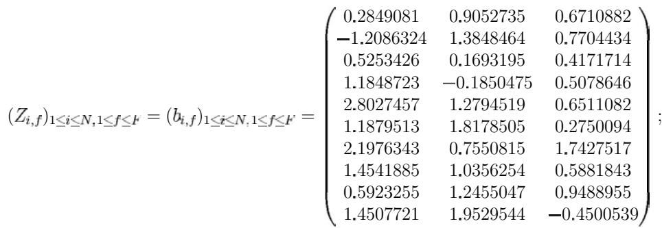That said, we need to fix the values for the $a$ 's, $b$ 's and the $\bar{A}_f$ 's. In our experiment, we choose the following values $N = 10$, $F = 3$, $S = \exp$ (so that the $b$ 's are the Z-scores), and: $$ (Z _ {i, f}) _ {1 \leq i \leq N, 1 \leq f \leq F} = (b _ {i, f}) _ {1 \leq i \leq N, 1 \leq f \leq F ^ {\prime}} = \left( \begin{array}{c c c} 0. 2 8 4 9 0 8 1 & 0. 9 0 5 2 7 3 5 & 0. 6 7 1 0 8 8 2 \\- 1. 2 0 8 6 3 2 4 & 1. 3 8 4 8 4 6 4 & 0. 7 7 0 4 4 3 4 \\0. 5 2 5 3 4 2 6 & 0. 1 6 9 3 1 9 5 & 0. 4 1 7 1 7 1 4 \\1. 1 8 4 8 7 2 3 & - 0. 1 8 5 0 4 7 5 & 0. 5 0 7 8 6 4 6 \\2. 8 0 2 7 4 5 7 & 1. 2 7 9 4 5 1 9 & 0. 6 5 1 1 0 8 2 \\1. 1 8 7 9 5 1 3 & 1. 8 1 7 8 5 0 5 & 0. 2 7 5 0 0 9 4 \\2. 1 9 7 6 3 4 3 & 0. 7 5 5 0 8 1 5 & 1. 7 4 2 7 5 1 7 \\1. 4 5 4 1 8 8 5 & 1. \text {0 .} \text {3} \text {6} \text {2} \text {5} \text {4} \text {7} \text {8} \text {9} \text {5} \\\text {0 .} \text {5} \text {9} \text {2} \text {3} \text {2} \text {5} \text {5} \text {4} \text {7} \text {8} \text {9} \text {5} \\\text {1 .} \text {4} \text {5} \text {0} \text {7} \text {2} \text {1} \text {3} \text {6} \text {9} \text {5} \\\text {1 .} \text {4} \text {5} \text {0} \text {7} \text {2} \text {1} \text {3} \text {6} \text {9} \text {5} \\\text {1 .} \text {4} \text {5} \text {0} \text {7} \text {2} \text {1} \text {3} \text {6} \text {9} \text {5} \\\text {1 .} \text {4} \text {5} \text {0} \text {7} \text {2} \text {1} \text {3} \text {\Delta} _ {\cdot , i}, \\& & - _ {\cdot , i}. \end{array} \right); $$ $$ (\bar {A} _ {f}) _ {1 \leq f \leq F} = \left(\frac {1}{N} \sum_ {i = 1} ^ {N} Z _ {i, 1}, (1 + 1 / 1 0 0) \frac {1}{N} \sum_ {i = 1} ^ {N} Z _ {i, 2}, (1 + 2 / 1 0 0) \frac {1}{N} \sum_ {i = 1} ^ {N} Z _ {i, 3}\right); $$ $$ \left(a _ {i, f}\right) _ {1 \leq i \leq N, 1 \leq f \leq F} = (\bar {A} _ {f}) _ {1 \leq f \leq F} - \left(b _ {i, f}\right) _ {1 \leq i \leq N, 1 \leq f \leq F}. $$ For the Z-scores, we took realisations of a Gaussian random variable of mean 1 and standard deviation 0.9. The Newton-Raphson iterative method has been used to reach for a minimum, and the objective function $\mathcal{O}$ has been set to be $$ \mathcal {O} \left(\alpha_ {1}, \alpha_ {2}, \alpha_ {3}\right) = \sum_ {f = 1} ^ {3} \left| \mathcal {F} _ {f} \left(\alpha_ {1}, \alpha_ {2}, \alpha_ {3}\right) \right|. $$ More specifically, we have generated 1000 initial enhancements, each given by the realisation of a Gaussian random vector of mean 1 and standard deviation 0.5. We have also done the exercise with another series of 1000 simulations, but with mean 10 and standard deviation 5, and another 1000 with mean 100 and standard deviation 50. The roots found are systematically the same for all the 3000 simulations: $$ \left(\alpha_ {1}, \alpha_ {2}, \alpha_ {3}\right) = (- 0. 0 0 2 8 0 2 9 7 4, 0. 0 4 4 5 9 9 9 1, 0. 0 6 3 7 3 9 2 7). $$ At this point, the value of the $\mathcal{F}_f$ 's are of order 10-15, which is of the precision of the machine. Finally, the estimation precision is of the order 10-15, also reaching the machine precision. The number of iterations varies, depending on the initial enhancement, but never reaches 1000. Within this set of parameters, we start to meet numerical issues if the initial enhancement have too negative values. For instance, if the initial value are $(-1, -1, -1)$, the roots found are $$ \left(\alpha_ {1}, \alpha_ {2}, \alpha_ {3}\right) = (- 1 0. 1 7 4 9 9, - 1 1. 1 1 8 3 5, - 1 2. 9 0 9 3 9), $$ but the magnitude order for the values of the functions $\mathcal{F}_f$ 's at this point are of order $10^{-6}$ (same for the estimated precision), which shows this point is a local minimum for the objective function, but clearly not the global one. This shows the limitation of the numerical method, and further numerical studies would perhaps be needed to further illustrate the main result of this paper.    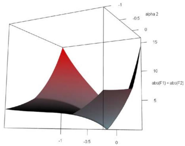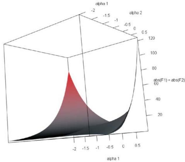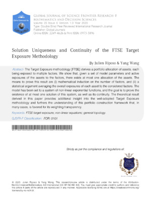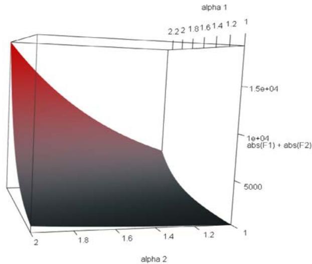 Figure 1: Plot of the objective function $|\mathcal{F}_1(\alpha_1, \alpha_2)| + |\mathcal{F}_2(\alpha_1, \alpha_2)|$ versus $\alpha_1$ and $\alpha_2$ around the unique root (-0.0002063940, 0.02590912). We conclude this part with an additional graphical illustration. We choose $F' = 2$ and $N = 10$, and the Z-scores are the first two columns of the above Z-scores matrix. The found that the root is given by $$ \left(\alpha_ {1}, \alpha_ {2}\right) = (- 0. 0 0 0 2 0 6 3 9 4 0, 0. 0 2 5 9 0 9 1 2), $$ with values for the $\mathcal{F}_f$ 's of order $10^{-14}$ (same for the estimated precision). Figure 2 plots the 3D-surface of the objective function $|\mathcal{F}_1(\alpha_1, \alpha_2)| + |\mathcal{F}_2(\alpha_1, \alpha_2)|$ versus $\alpha_1$ and $\alpha_2$. As shown, when we leave the neighbourhood of the root, the objective function significantly increases from 0. We also note that some convexity appears in the negative values of $\alpha_1$ and $\alpha_2$ (see the bottom of the surface in the top right figure), showing that another local minimum, which is not the global one, could be reached using the Newton-Raphson method once the initial enhancement is sufficiently close to it; but it is unlikely to be found in this area.      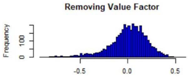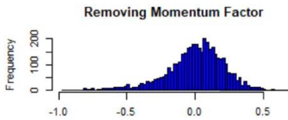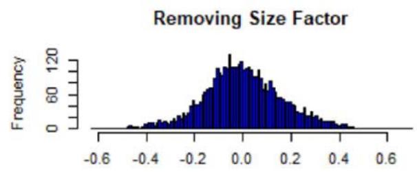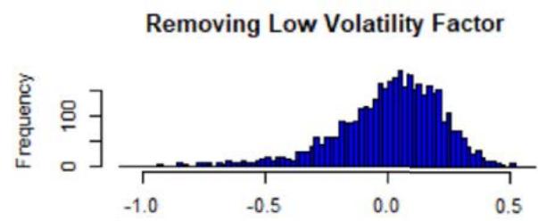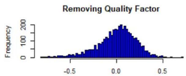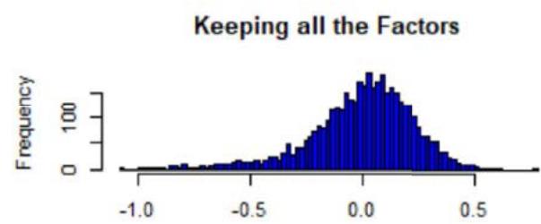 Figure 2: Histograms of the sum of Z-scores weighted by the root numbers (five factors), from the FTSE All-World Index data (see Equation (18)). The numbers are comprised between -1 and 1, and centered around 0 with a standard deviation of approx. 0.5. The 'symmetry' suggests that the Mean approximation is a statistical argument. The presence of extreme values also suggests that the Mean approximation is not a necessary condition to have uniqueness, but sufficient only. To illustrate the numerical example using practical data, we use FTSE All-World index as the opportunity set. It includes listed companies from both developed and emerging markets, which are classified as large and mid size companies by market cap (for details, see [GEIS]). This index represents a portfolio with around $N \approx 4100$ equity instruments, and $F = 5$ factors, Value, Momentum, Size, Low Volatily, and Quality. The proof of Theorem 1 is using the Mean approximation, see Definition 1. Testing this approximation is important. We note that the strengths $a$ priori are dependent variables. For the given set of parameters imposed by the data, the strengths $(\alpha_{h}^{*})_{h\in \{1,\ldots,5\}}$ designate the unique solution of the system found at rebalance date 21/03/2022. Fixing factor $f\in \{1,2,\dots,5\}$, we know that the numbers $(\alpha_h^*)_{h\in \{1,\dots,5\} \setminus \{f\}}$ are functions of $\alpha_{f}^{*}$. Bearing Equation (14) in mind, we see that $$ \bar {\mathcal {F}} _ {f} (\alpha_ {f} ^ {*} + \alpha) = \sum_ {i = 1} ^ {N} \left(a _ {i, f} \mathrm {e} ^ {\sum_ {l = 1} ^ {F} z _ {i, l} \alpha_ {l} ^ {*} (\alpha_ {f} ^ {*} + \alpha)} l \neq f\right) \mathrm {e} ^ {Z _ {i, f} \alpha_ {f} ^ {*} + Z _ {i, f} \alpha}, $$ where $\alpha$ is a perturbation of the solution strength $\alpha_{f}^{*}$. Thus, a proxy to have access to the variation of the numbers $(\alpha_{h}^{*})_{h\in \{1,\ldots,5\} \setminus \{f\}}$ with respect to $\alpha_{f}^{*}$ is to replace $Z_{i,f}\alpha$ with $\alpha \alpha_{f}^{*}$: $Z_{i,f}\alpha$ is itself a perturbation, so as $\alpha \alpha_{f}^{*}$. In fact, the proxy consists in identifying the perturbation of $\alpha$ for the Z-score with the variation of $\alpha_{f}^{*}$. Bearing this in mind, it is interesting to focus on the quantity $\mathcal{H}_f$, function of the perturbation $\alpha$ of the Z-score $Z_{i,f}$ 's and given by $$ \mathcal {H} _ {f} (\alpha) = \sum_ {\substack {h = 1 \\h \neq f}} ^ {F} Z _ {i, h} \alpha_ {h} ^ {*} (\alpha), \tag{18} $$ where we excluded a given factor $f$ in the sum, and where $\alpha_{h_k}^*(\alpha)$ is the strength found after the Z-scores are perturbed by $\alpha$. In Figure 2, we plotted the histogram of the sum $\mathcal{H}_f$ (one realization for one value of $\alpha$, chosen as realized Gaussian random variables of parameters $(0,1)$ (size of sample: 1000)), and we see that most of the values are concentrated around 0, but there are more extreme ones (even if $< 1$ ). The root uniqueness may not need the Mean approximation. We now focus on Equation (16). First, Figure 3 shows the $\mathcal{H}_f$ 's (see Equation (18)) with respect to $\alpha$. For the chosen instrument, the linear approximation is quite correct as witnessed by the $R^2$ values, see Figure 3. However, Figure 4 shows the same plots for another instrument, and the linear approximation is not convincing. We calculated the averaged $R^2$ for all the factors and for all the instruments, at all the rebalance dates between 2015 and 2022 (8 samples). It is given by 0.748, with a standard deviation of 0.300. As specified in Section 5, the order-3 polynomial is an excellent approximation for all the factors, instruments, and considered years. We also calculated the averaged $R^2$, which is 0.998, with a standard deviation of 0.015. ## VII. CONCLUSION In this paper, we have explained the Target Exposure methodology, abundantly used by the index industry and passive investment community. The Target Exposure derives an allocation of considered assets, allowing an investor to build portfolios that are exposed to various factor risks. It provides the investors a construction tool that gives transparency and intuition inherited from traditional tiling. Weighting transparency is a growing consideration of the passive investment community, especially when it includes sustainable investment goals such as ESG or carbon emission intensity. The discussion on the uniqueness of this allocation for a given set of exposures targets furthers our understanding of the target exposure framework.      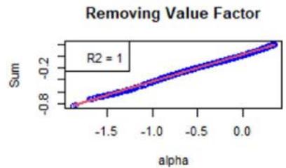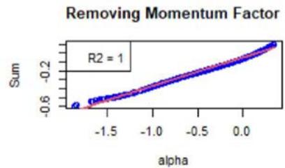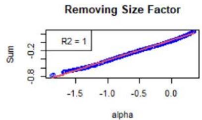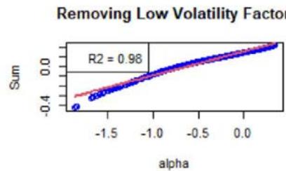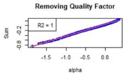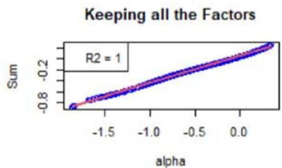 Figure 3: Scatter plot of the sums as defined by the $\mathcal{H}_f$ 's (see Equation (18)) vs $\alpha$ defined around 0, for a chosen instrument for which the linear approximation (see Equation (16)) is good. We have first reduced the Target Exposure model to a system of non-linear exponential functions. We have fully established the uniqueness of the solution in case we've considered only one factor. Then, as the most difficult part, we have proven the uniqueness of the solution for any number of factors, under a useful statistical approximation, the Mean approximation. Consisting in averaging the exposures of each asset to their factors overall, this approximation allowed completing the mathematical induction approach on the number of factors: we were able to show that there exists at most one allocation for a given considered universe of parameters, reduced to given compact sets of multi-dimensional real vector space. The fact that the result is true for any compact set is not restrictive at all: if the compact set is too small, the unique solution will unlikely be contained in it. Thus, it is suggested to move the compact set in the universe of parameters, or increase its size, until finding the solution. We see that compact sets here are the mathematical justification for playing with the set of parameters, in the research of the unique possible allocation. Tilting is one of the most common for use modern portfolio construction methodologies. Target Exposure aims to extend the tilting capability to incorporate explicit ex-ante outcomes while keeping the transparent weighting formulation. The extension to Target Exposures introduces a system of non-linear equations. The discussion of the root of this system of equations, particularly its uniqueness, has presented us with an interesting and challenging task. This paper has laid the groundwork for potential deeper dive into this system. While multiple solutions of such a system would further lead to possible discussions on different portfolios yielding identical investment objectives, our study so far has shown that such a scenario is not likely. The research proposed in this paper shows that the system underpinned by the Target Exposure problem has at most one real and continuous solution. 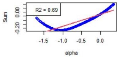 Removing Value Factor 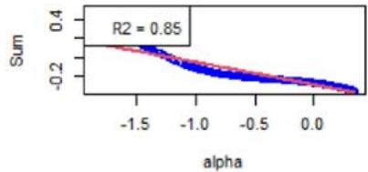 Removing Momentum Factor 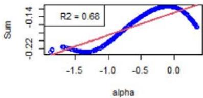 Removing Size Factor 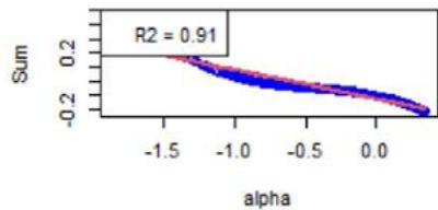 Removing Low Volatility Factor 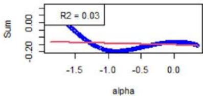 Removing Quality Factor 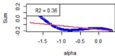 Figure 4: Same as Figure 3 but for another instrument, for which the linear approximation (see Equation (16)) is not a good approximation. However, for all the instruments, the order-3 polynomial approximation is a very good approximation. ### ACKNOWLEDGMENTS We are very thankful for the discussions we had with the Index Research & Design Team at London Stock Exchange Group. #### Conflict of Interest The authors declare no conflict of interest. The views expressed in this paper are those of the authors and do not necessarily reflect the views and policies of LSEG - FTSE. #### Data Availability Statement Data available on request due to privacy/ethical restrictions.

Generating HTML Viewer...

References

32 Cites in Article
Diyashvir Babajee (2015). Some Improvements to a Third Order Variant of Newton’s Method from Simpson’s Rule.
D Babajee,M Dauhoo,M Darvishi,A Barati (2008). A note on the local convergence of iterative methods based on Adomian decomposition method and 3-node quadrature rule.
Jennifer Bender,Taie Wang (2016). Can the Whole Be More Than the Sum of the Parts? <i>Bottom-Up versus Top-Down Multifactor Portfolio Construction</i>.
R French Latent Factors in Equity Returns: How Many Are There and What Are They?.
R French Redefining Growth: Using analyst forecasts to transcend the value growth dichotomy.
B Freno,K Carlberg (2019). Machine-learning error models for approximate solutions to parameterized systems of nonlinear equations.
Darren Butterworth,Phil Holmes (2001). The hedging effectiveness of stock index futures: evidence for the FTSE-100 and FTSE-mid250 indexes traded in the UK.
Khalid Ghayur,Ronan Heaney,Stephen Platt (2018). Constructing Long-Only Multifactor Strategies: Portfolio Blending vs. Signal Blending.
M Capinski,E Kopp (2014). Portfolio Theory and Risk Management.
A Golbabai,M Javidi (2007). A new family of iterative methods for solving system of nonlinear algebric equations.
R Grinold,R Kahn (1999). Active Portfolio Management: A Quantitative Approach for Producing Superior Returns and Selecting Superior Returns and Controlling Risk.
Wenrui Hao (2021). A gradient descent method for solving a system of nonlinear equations.
G Jameson (2006). Counting zeros of generalised polynomials: Descartes’ rule of signs and Laguerre’s extensions.
J Riposo,E Klepfish Notes on the Convergence of the Estimated Risk Factor Matrix in Linear Regression Models.
Harry Markowitz (1952). PORTFOLIO SELECTION*.
J Choy,M Dutt,J Garcia-Zarate,K Gogoi,B Johnson (2022). A global Guide to Strategic-Beta Exchange-Traded Products Morningstar.
M Noor,M Waseem (2009). Some iterative methods for solving a system of nonlinear equations.
Russell Unknown Title.
J Riposo (2018). Some Spectral Asset Management Methods.
R Rizk-Allah] Rizk-Allah (2021). A quantum-based sine cosine algorithm for solving general systems of nonlinear equations.
W Sharpe The Sharpe Ratio.
Y Wang,P Gunthorp,D Harris EU Paris-Aligned and Climate Transition Benchmarks: A Case Study.
W Forst,D Hoffmann (2010). Optimization -Theory and Practice.
Explore published articles in an immersive Augmented Reality environment. Our platform converts research papers into interactive 3D books, allowing readers to view and interact with content using AR and VR compatible devices.
Your published article is automatically converted into a realistic 3D book. Flip through pages and read research papers in a more engaging and interactive format.
The Target Exposure methodology [FTSE] derives a portfolio allocation of assets, each being exposed to multiple factors. We show that, given a set of model parameters and active exposures of the assets to the factors, there exists at most one allocation of the assets. The means to prove this result are (i) mathematical induction on the number of factors, and (ii) a statistical argument averaging the overall exposures of each asset to the considered factors. The model has been set to a system of non-linear exponential functions, and the goal is to prove the existence of at most one solution of this system, as well as its continuity. The theoretical result derived in this paper provides additional insight into the well-adopted Target Exposure methodology and furthers the understanding of this portfolio construction framework that, in many cases, is favored for its weighting transparency.
Our website is actively being updated, and changes may occur frequently. Please clear your browser cache if needed. For feedback or error reporting, please email [email protected]
Thank you for connecting with us. We will respond to you shortly.