## I. INTRODUCTION Complex dynamics usually refers to nonlinearly coupled systems. These divide into two main classes: a) the autonomous models, whose behavior depend on specific control parameters -such as the case of an unstable laser [1], and the Lorenz model of turbulence [2]- and b) the non-autonomous systems that respond nonlinearly to some harmonic excitation, externally supplied by an adequate mechanism. The dynamical properties of these systems usually rely on computer simulations. Numerous examples have been put forward to demonstrate the complex-and unpredictable- behavior of nonlinear models that are generally described in terms of coupled differential equations, which contain -at least- one nonlinear term [3-6]. However, no report has expanded the analysis of the undamped harmonic oscillator, externally driven with harmonic excitations. The usual approach to hold this simple model is limited to analytical ingredients that have become standard in introductory courses at the undergraduate level. The commonly accepted point is that sinusoidal excitations yield comparative sinusoidal responses. Our investigations reveal that such a conclusion is incomplete to explain the wealth of solutions outputting from the system. The harmonic oscillator is -par excellence- the fundamental dynamical system, which introduces at the very first academic lectures of physics and mathematics [7-18]. The study of the autonomous scheme usually goes along with the introduction of second-order differential equations in mathematics, and the study of small-amplitude oscillations in physics, whereas the non-autonomous case is delayed until the undergraduate years, imparting in the more specific classes of mechanics and vibrations. Its properties are so largely recognized that trying to bring new elements of analysis may seem difficult, if not impossible. Yet, despite its universally acknowledged properties, we shall reveal new outcomes and features that have never been disclosed before. The new findings are based on an overlooked solution that plays an essential role in orbit modelling. Even though the new approach does not question the model's main property, i.e., its intrinsic resonant phenomenon, it unveils further complexities. The disclosures arise from extensive computer analysis. The numerical solutions are shown to follow their analytical counterparts, which are straightforwardly derived from the introduction of the overlooked solution. The study reveals a wealth of phase-space trajectories, with sequences that stem from locking and beating mechanisms between the forcing and the resonant frequencies. These phenomena retrieve with direct numerical simulations while recovering -with staggering precision- from the new analytical ingredients. The presentation develops according to the following hierarchy. After recalling the properties of the autonomous harmonic oscillator in Sec. II, the non-autonomous system is presented in Sec. III. Sec. IV deals with irregular signals and a periodic trajectories, while some locking phenomena and period-doubling sequences are presented in Sec. V. A few concluding remarks follow in Sec. VI, and three appendixes are integrated to give comprehensive accounts of the primary analytical aspects. ## II. THE AUTONOMOUS HARMONIC ### Oscillator: The Pendulum and Mass-SPRING EXAMPLES The oscillatory movement of a simple pendulum of length $l$ describes with the second-order differential equation. $$ \frac{d^{2}\theta}{dt^{2}} + \frac{g}{l} \sin(\theta) = 0 \tag{1a} $$ $$ \frac {d ^ {2} \theta}{d t ^ {2}} + \omega_ {0} ^ {2} \sin (\theta) = 0 \tag {1b} $$ where $$ \omega_ {0} = 2 \pi f _ {0} = \sqrt {\frac {g}{l}} \tag {1c} $$ is the free-oscillator pulsation (angular frequency), and $f_0$ its natural frequency. For small enough $\theta$, i.e., $\theta \leq \frac{\pi}{18}$, $\sin(\theta) \cong \theta$ (it takes a pocket calculator to check that $\sin\left(\frac{\pi}{18}\right) \cong \frac{\pi}{18}$ ), the equation becomes $$ \frac {d ^ {2} \theta}{d t ^ {2}} + \omega_ {0} ^ {2} \theta = 0 \tag {2a} $$ Whose solution reads $$ \theta = \theta_{0} \cos(\omega_{0} t) \tag{2b} $$ The pendulum oscillates with the angular velocity $$ \frac{d\theta}{dt} = -\omega_0 \theta_0 \sin(\omega_0 t) = \omega_0 \theta_0 \cos\left(\omega_0 t + \frac{\pi}{2}\right) \tag{2C} $$ Showing a $\frac{\pi}{2}$ phase difference between the velocity and the displacement. The elements of analysis apply to the case of a free mass-spring oscillator. The mass small movement $x(t)$ around the position of equilibrium satisfies $$ \frac {d ^ {2} x}{d t ^ {2}} + \omega_ {0} ^ {2} x = 0 \tag {3a} $$ whose solution reads, $$ x = x _ {0} \cos (\omega_ {0} t), \tag {3b} $$ for the displacement, and $$ v (t) = \frac {d x}{d t} = - \omega_ {0} x _ {0} \sin (\omega_ {0} t) = v _ {0} \cos (\omega_ {0} t + \frac {\pi}{2}) \tag {3c} $$ for its speed. From Eqs (3b) and (3c), we readily derive $$ \left(\frac {x}{x _ {o}}\right) ^ {2} + \left(\frac {\mathrm {v}}{\mathrm {v} _ {o}}\right) ^ {2} = 1 \tag {3d} $$ i.e., the equation of an ellipse, which represents the system's trajectory in phase space. If the maximum position and maximum speed have the same absolute values, the phase space orbit transforms into a circle. The orbit exact shape depends on the precise initial conditions, i.e., on $x_0$ and $v_0$. Figure 1 depicts two examples corresponding to a) $x_0 = 1$, $\omega_0 = 1$, and b) $x_0 = 1$, $\omega_0 = 2$. 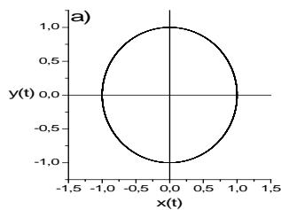In the figures, $y(t) = v(t) = \frac{dx}{dt}$  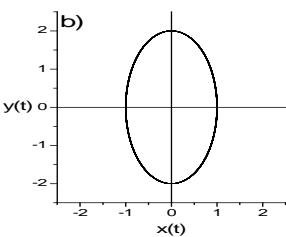 Figure 1: Phase space trajectories obtained with a) $x_0 = 1$, $\omega_0 = 1$ (circular orbit), and b) $x_0 = 1$, $\omega_0 = 2$ (elliptical trajectory). ## III. THE NON-AUTONOMOUS SYSTEM When some sinusoidal excitation of the form $f(t) = F\cos (\omega t)$ is supplied to the harmonic oscillator not undergoing any damping force, the mass movement describes with $$ \frac {d ^ {2} x}{d t ^ {2}} + \omega_ {0} ^ {2} x = F \cos (\omega t) \tag {4a} $$ As introduced in mechanics-and-vibrations lessons, the usual method of solving such an equation away from resonance, is to consider a response of the same form as the excitation, i.e. $$ x (t) = A \cos (\omega t + \varphi) \tag {4b} $$ Where amplitude $A$ and phase $\varphi$ are coefficients that must be evaluated. Plugging Eq. (4b) into Eq. (4a), yields $$ - A \omega^ {2} \cos (\omega t + \varphi) + A \omega_ {0} ^ {2} \cos (\omega t + \varphi) = F \cos (\omega t) \tag {4c} $$ i.e., $$ \begin{array}{l} \left[ \omega_ {0} ^ {2} - \omega^ {2} \right] A \cos (\omega t) \cos (\varphi) - \left[ \omega_ {0} ^ {2} - \omega^ {2} \right] A \sin (\omega t) \sin (\varphi) = \\F \cos (\omega t) \tag {4d} \\\end{array} $$ implying $$ \left[ \omega_ {0} ^ {2} - \omega^ {2} \right] A \sin (\varphi) = 0 $$ and $$ \left[ \omega_0^2 - \omega^2 \right] A \cos(\omega t) \cos(\varphi) = F $$ Since $\omega \neq \omega_0$, and $A \neq 0$, we are left with $\varphi = 0 \mod \pi$, and $$ A = \frac {F}{\omega_ {0} ^ {2} - \omega^ {2}} \tag {4g} $$ $$ x (t) = \frac {F}{\omega_ {0} ^ {2} - \omega^ {2}} \cos (\omega t) \tag {4h} $$ For the displacement, and $$ \frac {d x}{d t} = - \frac {F \omega}{\omega_ {0} ^ {2} - \omega^ {2}} \sin (\omega t) \tag {4i} $$ for its speed. Note that the response is linearly correlated to the excitation, i.e. $$ x(t) = A(\omega)f(t) $$ Eqs (4h) and (4i) carry the well-known phenomenon of resonance, which occurs at $\omega = \omega_0$. The resonance curve, represented in Fig. 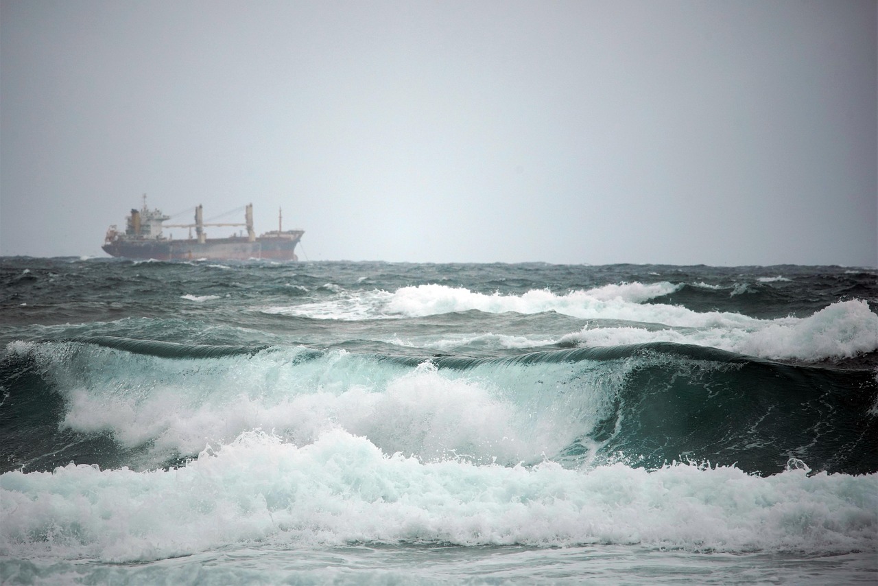2, with the parameters $\omega_0 = 1$, and $F = 1$, shows the notable infinite-amplitude-catastrophe that occurs at $\omega = \omega_0$, and which was responsible for famous disasters in the past: - On April 18, 1850, in Angers (France), a military unit crossing in cadenced steps a suspension bridge spanning the Maine river caused its destruction. - On November 7, 1940, six months after its inauguration, the Tacoma bridge (USA) was destroyed by the effects of gusts of winds, which - without being particularly violent $(60\mathrm{km / h})$ -were regular. 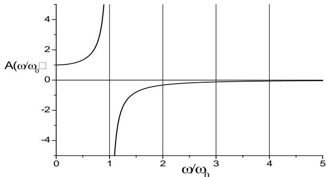 Figure 2: Resonance phenomenon which occurs when the driving frequency $f = \frac{\omega}{2\pi}$ equals the system's proper frequency $f_0 = \omega_0 / 2\pi$. To derive an expression for the growing amplitude at resonance, we must solve $$ \frac{d^{2}x}{dt^{2}} + \omega_{0}^{2}x = F\cos\left(\omega_{0}t\right)\tag{5a} $$ With the initial conditions, $x(0) = 0$, and $dx / dt = 0$, we are left with (see appendix A for details) $$ x (t) = \frac {F}{2 \omega_ {0}} t \cos (\omega_ {0} t) \tag {5b} $$ 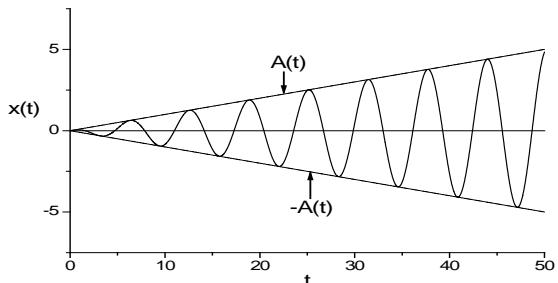 Figure 3: Displacement $x(t)$, simulated at resonance. Note the linearly growing amplitude towards infinity, following Eq. (5c). Showing a linearly growing amplitude with respect to $t$, an example of which is depicted in Fig. 3. $$ A(t) = \frac{F}{2\omega_0} t $$ Let us represent two typical solutions, describing with Eqs (4h) and (4i), away from resonance. Taking $F = 1$, $\omega = 0.5\omega_0$, and $\omega = 2\omega_0$, the corresponding trajectories depict with elliptical orbits, as portrayed in Fig. 4.  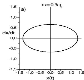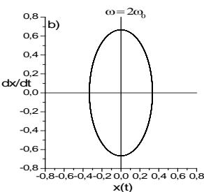 Figure 4: Elliptical orbits corresponding to Eqs (4h) and (4i), with a) $\omega = 0.5\omega_0$, and b) $\omega = 2\omega_{0}$ Whatever the parameter values and initial conditions, Eqs (4h) and (4i), describe elliptical or circular orbits. That is what we teach in fundamental physics and mathematics. However, the numerical analysis of Eq. (4a) tells a different story. To solve Eq. (4a) numerically, we introduce a $y$ variable and obtain two coupled differential equations of the first order $$ \frac {d x}{d t} = y \tag {6a} $$ $$ \frac {d y}{d t} = - \omega_ {0} ^ {2} x + F \cos (\omega t) \tag {6b} $$ It takes some basic numerical code, such as the second-or-fourth order Runge-Kutta algorithms, to solve Eqs (6). The simulated solution corresponding to $F = 1$, $\omega = 0.5\omega_0$, with the initial conditions $x(0) = 0$, and $y((0) = 0$ is represented in Fig. 5. To fully sense the ingredients of the solution, we depicted the time traces, the spectrum, and the phase-space portrait. It takes this first example to grab the difference between the orbits of Fig. 4 and that of Fig. 5d. The ellipse converting into a double-loop trajectory. Such a double-loop orbit usually characterizes nonlinear systems. Since no obvious nonlinearity seems to connect $x$ and $y$, in Eqs (6), one cannot but feel surprised by such an unanticipated nonlinear response: Fig. 5a clearly indicates that $x(t)$ is not a pure sinusoidal function. Therefore, it is not linearly related to $f(t)!$. Such a new and fundamental result is analytically derived in the following (see Eqs (8a) and (8c)).    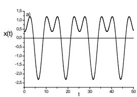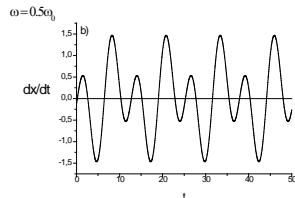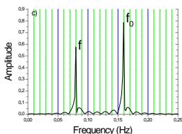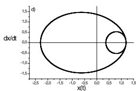 Figure 5: a) Displacement, b) speed, c) Fourier spectrum, and d) phase-space orbit, as simulated with Eqs (6), and an excitation frequency equal to half the natural one. Since we chose $\omega_0 = 1$, the fundamental frequency scales as $f_0 = \frac{1}{2\pi} \cong 0.16$. As represented in Fig. 6, at $\omega = 2\omega_0$ we retrieve the features of Fig. 5d, which was simulated at $\omega = 0.5\omega_0$. Such a resemblance is not limited to the present example. It clarifies with the full analytical solution, as henceforth demonstrated. 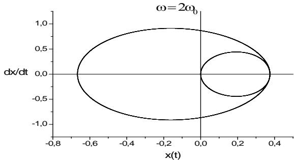 Figure 6: Phase-space orbit corresponding to $\omega = 2\omega_0$. Note the similarity with Fig. 5d. 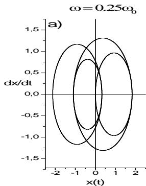Two other orbits, corresponding to $\omega = 0.25\omega_0$ and $\omega = 4\omega_0$ are represented in Fig. 7. Again, the two trajectories are similar.  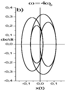 Figure 7: Simulated four-cycle orbits corresponding to a) $\omega = 0.25\omega_0$, and b) $\omega = 4\omega_0$. Note the similarity between the two trajectories. Indeed, due to their dependence on frequency, the amplitudes scale differently. Additional trajectories, corresponding to $\omega = 5\omega_0$ and $\omega = 10\omega_0$ are represented in Figs. 8 and 9. As expected, the Fourier spectrum of Fig. 8a indicates the presence of the natural and excitation frequencies. The temporal time trace of Fig. 9a points to some well-structured modulation effect, the low frequency $f_0 - f$ modulating the high pulsation signal $f_0 + f$ (see Appendix B for detailed analytical accounts).  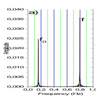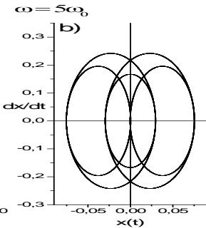 Figure 8: a) Fourier spectrum, and b) phase-space orbit, simulated with $\omega = 5\omega_0$. The trajectory is a fifth-order orbit. In view of these unusual and unexpected results, it becomes obvious that Eq. (4h) is partial, if not unsatisfactory. As discussed above, the commonly admitted solution to Eq. (4a) is Eq. (4h). However, such a solution is incomplete because it neglects the intrinsic properties of the autonomous system $$ \frac {d ^ {2} x}{d t ^ {2}} + \omega_ {0} ^ {2} x = 0 \tag {7a} $$ which must be added to Eq. (4h). Consequently, the complete solution should read (see Appendix A for details) 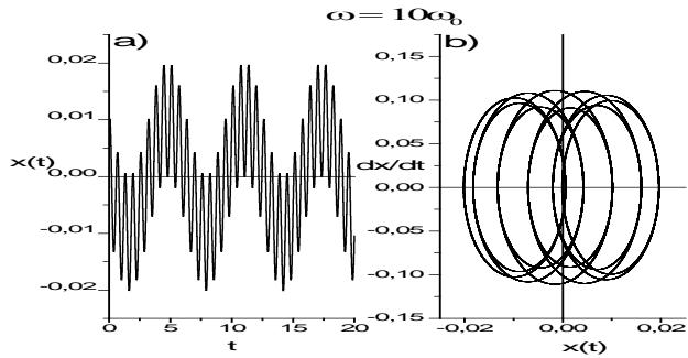 Figure 9: a) Displacement time trace in the form of modulated and modulating signals (see appendix B for details and formulations), and b) multi-loop (of the tenth order) trajectory, simulated with $\omega = 10\omega_0$. $$ x (t) = A \cos (\omega_ {0} t) + B \cos (\omega t) \tag {7b} $$ Which, when plugged into Eq. 4a, yields $$ -A\omega_0^2\cos(\omega_0 t) - \omega^2 B\cos(\omega t) + A\omega_0^2\cos(\omega_0 t) + B\omega_0^2\cos(\omega t) = F\cos(\omega t) \tag{7c} $$ $$ B = \frac{F}{\omega_ {0} ^ {2} - \omega^ {2}} \tag{7d} $$ $$ x (t) = A \cos (\omega_ {0} t) + \frac {F}{\omega_ {0} ^ {2} - \omega^ {2}} \cos (\omega t) \tag {7e} $$ Furthermore, with the initial condition $x(t) = 0$ at $t = 0$, Eq. (7e) converts into $$ x (t) = \frac {F}{\omega_ {0} ^ {2} - \omega^ {2}} \left(- \cos \left(\omega_ {0} t\right) + \cos (\omega t)\right) \tag {8a} $$ While the displacement velocity expands as $$ \frac {d x}{d t} = \frac {F}{\omega_ {0} ^ {2} - \omega^ {2}} \left(\omega_ {0} \sin (\omega_ {0} t) - \omega \sin (\omega t)\right) \tag {8b} $$ If the initial displacement changes into $x(t) = x_0$, at $t = 0$, then $x(t)$ writes [see appendix A] $$ x(t) = \left[ x_{0} - \frac{F}{\omega_{0}^{2} - \omega^{2}} \right] \cos(\omega_{0} t) + \frac{F}{\omega_{0}^{2} - \omega^{2}} \cos(\omega t) \tag{8c} $$ As one can see, whatever the initial conditions, the state of resonance is preserved through similar frequency dependent amplitudes.    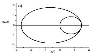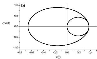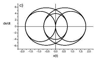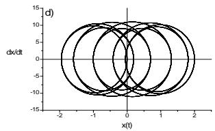 Figure 10: Phase space orbits describing with Eqs (8) and, a) $\omega = 0.5\omega_{0}$, b) $\omega = 2\omega_{0}$, c) $\omega = 5\omega_{0}$, and $\omega = 10\omega_{0}$. Note however that -as expected from the numerical solutions- we have analytically retrieved the nonlinear nature of $x(t)$ with respect to $f(t)$, since both Eq (8a) and Eq. (8c) write as combinations of two distinct functions $$ x (t) = A (\omega) f (t) + B (\omega) g (t) \tag {9} $$ This constitutes a major outcome of the present report. Such a fundamental result has never been highlighted in past studies. Most studies focused on the damped case, limiting the undamped one to its least ingredients. In so doing we all missed the main point about the nonlinear nature of the harmonic oscillator. Let us use the same examples as the simulated ones and represent the solutions for $f(t) = \cos (\omega t)$, $x(0) = 0$, and respectively $\omega = 0.5\omega_0$, $\omega = 2\omega_0$, $\omega = 5\omega_0$, and $\omega = 10\omega_0$. The corresponding trajectories are depicted in Fig. 10. Indeed, if one wants to compare the associated time traces, Eq (8a) perfectly describes the features of Figs 5a, 5b and 9a, or those of any other example, provided the two involved frequencies scale commensurately to prevent irregular signals and fuzzy aperiodic trajectories. As a last and compelling example pertaining to the validity of Eqs (8), let us solve the differential equation with $\omega = 3\omega_0$. The result is a -somewhat peculiar- three-orbit trajectory. Nonetheless, an exact replica generates with Eqs (8). It is represented in Fig. 11. Let us again note that a similar phase-space portrait obtains with $\omega = \omega_0 / 3$. 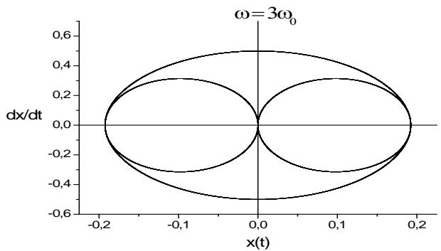 Figure 11: Analytical and numerical three-loop trajectory obtained with $\omega = 3\omega_0$, and, equivalently, with $\omega = \omega_0 / 3$ All these examples, and numerous others, demonstrate the validity of Eqs (8). A one-to-one comparison between the numerical and the analytical results does not call for supplementary comments, since a one-to-one correspondence obtains whatever the initial conditions or the driving frequency, as well as the forcing amplitude. $F$ and $\omega$ may consider as the two control parameters of the system. With respect to $\omega$, $F$ plays a minor role. One may therefore conclude that the general solution of the harmonic oscillator undergoing an external harmonic excitation of the form $F\cos(\omega t)$ contains both the exciting frequency $f$ and the system's natural frequency $f_0$. The above results are conclusive enough to include in future graduate and undergraduate programs that deal with oscillatory systems. The presented properties may serve as a simple introductory lesson to more complex dynamical systems. The above examples show some worth-mentioning symmetry properties. For instance, we found the same phase portraits with $\omega = 0.5\omega_0$, and $\omega = 2\omega_0$, as well as with $\omega = 0.25\omega_0$, $\omega = 4\omega_0$; $\omega = \frac{\omega_0}{3}$ and $\omega = 3\omega_0$. i.e., whenever $\omega = n\omega_0$ or $\omega_0 = n\omega$. In short, for any integer $n$ such that $\omega = n\omega_0$, similar trajectories obtain with $$ x (t) = - \cos (\omega_ {0} t) + \cos (n \omega_ {0} t) \tag {10a} $$ $$ \frac {d x}{d t} = \omega_ {0} \sin (\omega_ {0} t) - n \omega_ {0} \sin (n \omega_ {0} t) \tag {10b} $$ and $$ x (t) = - \cos \left(\frac {\omega}{n} t\right) + \cos (\omega t) \tag {10c} $$ $$ \frac{d x}{d t} = \frac{\omega}{n} \sin \left(\frac{\omega}{n} t\right) - \omega \sin (\omega t) \tag{10d} $$ It takes some simple graphical software to confirm these elements. Indeed, such a symmetric property is valid only for the case studied in this section, with the initial condition, $x(0) = 0$. ## IV. IRREGULAR SIGNALS AND APERIODIC TRAJECTORIES Irregular trajectories usually characterize more complex nonlinear systems through sequences of solutions ultimately ending in chaotic signals.  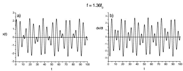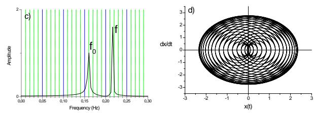 Figure 12: Analytical and numerical solution obtained with a driving frequency $f = 1.36f_{0}$, a) and b) irregular time traces, c) Fourier spectrum, and d) aperiodic trajectory. Let us represent the solution corresponding to Eq. (8c) by fixing the external frequency to incommensurately scale with the natural frequency. The example of Fig. 12 was simulated with $f = 1.36f_{0}$. The displacement and velocity time traces do not show any periodicity. The phase-space trajectory is multi-loop orbit with an infinite order. The orbit was simulated limiting the time span to $t = 100$. The more we increase $t$, the more surface the trajectory occupies. This is an indication of aperiodicity. The analytical descriptions of each graph in Fig. 12 obtain with the following expansions $$ x (t) = \cos \left(\omega_ {0} t\right) + \cos \left(1. 3 6 \omega_ {0} t\right) \tag {11a} $$ $$ \frac{d x}{d t} = - \omega_ {0} \sin (\omega_ {0} t) - 1.36 \omega_ {0} \sin (1.36 \omega_ {0} t) \quad (11b) $$ Again, outstanding similarities appear between the numerically simulated graphs of Fig. 12 and the analytical counterparts depicted in Fig. 13. Two frequency chaos has long been reported in complex systems [14]. However, to the best of our knowledge, it demonstrates here analytically for the first time, in the case of a harmonic oscillator. It takes Eqs (11), or any other expansions, with two incommensurate frequencies, to obtain irregular trajectories. As time flows, the orbits fill the entire plane, an indication of the aperiodic nature of the solution.  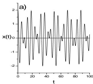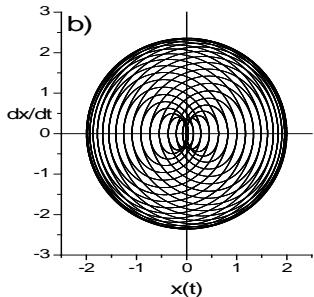 Figure 13: a) Irregular time trace, and b) aperiodic trajectory, obtained with Eqs (11). Noteworthy is the fact that slight changes in driving frequencies transform well-structured signals and orbits into aperiodic time traces and trajectories. These may consider as further examples of the famous butterfly effect, which demonstrates in other nonlinear systems, such as the Lorenz attractor [2, 15]. ## V. LOCKING PHENOMENA AND GENERATION OF SUB-HARMONIC SEQUENCES The sequence of period-doubling-or, equivalently, subharmonic cascading- is known in nonlinear dynamics as a route towards deterministic chaos [15]. Phase space trajectories with period doubling sequences also characterize the forced harmonic oscillator, as hereafter demonstrated in several cases with distinct control parameters and initial conditions. a) Period doubling sequence generated with $f(t) = 0.1 \sin (\omega t), \omega_0 = 1,$ and $x_0 = 0$. In this case, the solution expands into (see Appendix A) $$ x (t) = \frac {f}{\omega_ {0} ^ {2} - \omega^ {2}} - \frac {\omega}{\omega_ {0}} \sin (\omega_ {0} t) + \sin (\omega t) \tag {12a} $$ $$ y (t) = \frac {d x}{d t} = \frac {F \omega}{\omega_ {0} ^ {2} - \omega^ {2}} \left(- \cos \left(\omega_ {0} t\right) + \cos (\omega t)\right) \tag {12b} $$ The trajectories obtained both numerically and analytically, successively with $\omega = 2\omega_0$ (period one), $\omega = 1.5\omega_0$ (period two), $\omega = 1.25\omega_0$ (period four), and $\omega = 1.21\omega_0$ (aperiodic, the driving and natural frequencies scale incommensurately), are represented in Fig. 14. The full sequence of period doubling towards resonance generates with $$ \omega_ {1} = 2 \omega_ {0}, $$ $$ \omega_ {2} = 2 \omega_ {0} - \frac {1}{2} \omega_ {0}, $$ $$ \begin{array}{l} \omega_ {4} = \omega_ {2 ^ {2}} = 2 \omega_ {0} - \left(\frac {1}{2} + \left(\frac {1}{2}\right) ^ {2}\right) \omega_ {0}, \\\omega_ {8} = \omega_ {2 ^ {3}} = 2 \omega_ {0} - \left(\frac {1}{2} + \left(\frac {1}{2}\right) ^ {2} + \left(\frac {1}{2}\right) ^ {3}\right) \omega_ {0}, \\\end{array} $$ ··· $$ \omega_ {2 ^ {n}} = 2 \omega_ {0} - \left(\frac {1}{2} + \left(\frac {1}{2}\right) ^ {2} + \left(\frac {1}{2}\right) ^ {3} + \dots \left(\frac {1}{2}\right) ^ {n}\right) \omega_ {0}, \omega_ {2 ^ {\infty}} = \omega_ {0} $$ (resonance (aperiodic)). Each cycle of the sequence generates with Eqs (12). Note that $$ \begin{array}{l} \sum_ {n = 1} ^ {n} \frac {1}{2 ^ {n}} = \frac {1 - \left(\frac {1}{2}\right) ^ {n + 1}}{1 - \frac {1}{2}} - 1 = 1 - \left(\frac {1}{2}\right) ^ {n}, \\\omega_ {2 ^ {n}} = 2 \omega_ {0} - \left(1 - \left(\frac {1}{2}\right) ^ {n}\right) \omega_ {0} = \left(1 + \left(\frac {1}{2}\right) ^ {n}\right) \omega_ {0}, \\\end{array} $$ and $$ \begin{array}{l} \omega_ {0} ^ {2} - \omega_ {2 ^ {n}} ^ {2} = \omega_ {0} ^ {2} - \left(1 + \left(\frac {1}{2}\right) ^ {n}\right) ^ {2} \omega_ {0} ^ {2} = - \left(2 \left(\frac {1}{2}\right) ^ {n} + \left(\frac {1}{2}\right) ^ {2 n}\right) \omega_ {0} ^ {2} = \\- \left(\frac {1}{2}\right) ^ {n - 1} \left(1 + \left(\frac {1}{2}\right) ^ {n + 1}\right) \omega_ {0} ^ {2}. \\\end{array} $$ Also note that the state of resonance is reached at $\omega_{2^{\infty}} = \left(1 + \left(\frac{1}{2}\right)^{\infty}\right)\omega_{0} = \omega_{0}$. The complete sub-harmonic cascade depicts - and predicts- analytically with the following formulas $$ x _ {2 ^ {n}} (t) = \frac {F}{\omega_ {0} ^ {2} - \omega_ {2 ^ {n}} ^ {2}} \left(- \frac {\omega_ {2 ^ {n}}}{\omega_ {0}} \sin (\omega_ {0} t) + \sin (\omega_ {2 ^ {n}} t)\right) \tag {13a} $$ $$ y _ {2 ^ {n}} (t) = \frac {F \omega_ {2 ^ {n}}}{\omega_ {0} ^ {2} - \omega_ {2 ^ {n}} ^ {2}} \left(- \cos \left(\omega_ {0} t\right) + \cos \left(\omega_ {2 ^ {n}} t\right)\right) \tag {13b} $$ $$ With \omega_{2^{n}} = \left(1 + \left(\frac{1}{2}\right)^{n}\right) \omega_{0}, \, n = 0,1,2,3\dots $$    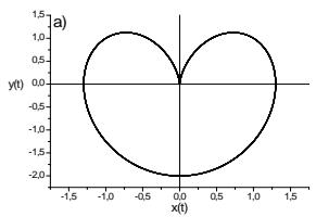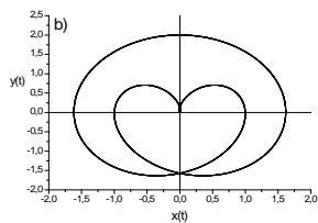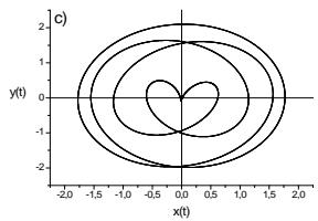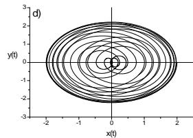 Figure 14: Period doubling sequence, analytically replicated with a) $\omega = 2\omega_0$ (period one), b) $\omega = 1.5\omega_0$ (period two), c) $\omega = 1.25\omega_0$ (period four), and d) $\omega = 1.21\omega_0$ (aperiodic orbit). The order of the trajectory corresponds to the value of $2^n$. For example, $2^0 = 1$ (period one), $2^2 = 4$ (period four), $2^3 = 8$ (period eight), $2^4 = 16$ (period sixteen), etc. According to Eqs (13), the period-8 trajectory follows $$ x _ {8} (t) = - \frac {6 . 4}{1 7} (- 1. 1 2 5 \sin (t) + \sin (1. 1 2 5 t)) \tag {14a} $$ $$ y _ {8} (t) = - \frac {7 . 2}{1 7} (- \cos (t) + \cos (1. 1 2 5 t)) \tag {14b} $$ where $\omega_{8} = \left(1 + \left(\frac{1}{2}\right)^{3}\right)\omega_{0} = \frac{9}{8}\omega_{0}$. We leave the reader with the simple task to replicate the corresponding orbit with any graphical software to confirm the associated periodicity. Indeed, one may -for the purpose of corroboration- confirm that exact replicas of the trajectories generate, as well, with numerical simulations of Eqs. (6). b) Period doubling sequence generated with $f(t) = 0.1 \sin (\omega t), \omega_0 = 1,$ and $x_0 = 1$. In this case, the solution expands into (see Appendix A) $$ x (t) = \frac {F}{\omega_ {0} ^ {2} - \omega^ {2}} \left(- \frac {\omega}{\omega_ {0}} \sin (\omega_ {0} t) + \sin (\omega t)\right) + x _ {0} \cos (\omega_ {0} t) (1 5 a) $$ $$ y (t) = \frac{d x}{d t} = \frac{F \omega}{\omega_ {0} ^ {2} - \omega^ {2}} \left(- \cos \left(\omega_ {0} t\right) + \cos (\omega t)\right) - x _ {0} \sin (\omega_ {0} t) \tag{15b} $$ The trajectories generated both numerically and analytically, successively with $\omega = 2\omega_0$ (period one), $\omega = 0.5\omega_0$ (period two), $\omega = 0.75\omega_0$ (period four) and $\omega = 0.875\omega_0$ (period eight) are represented in Fig. 15.    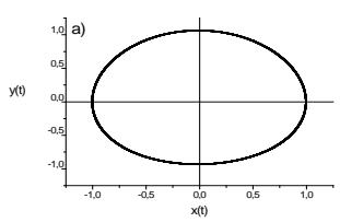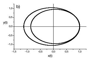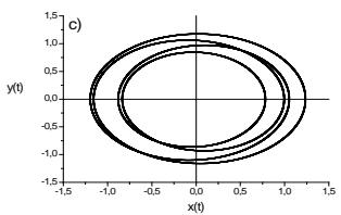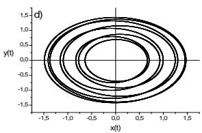 Figure 15: Period doubling sequence analytically replicated with a) $\omega = 2\omega_0$ (period one), b) $\omega = 0.5\omega_0$ (period two), c) $\omega = 0.75\omega_0$ (period four), and d) $\omega = 0.875\omega_0$ (period eight). c) Period doubling sequence generated with $f(t) = 0.1 \cos (\omega t)$, $\omega_0 = 1$, and $x_0 = 0$. The solution is described with $$ x (t) = \frac {0 . 1}{1 - \omega^ {2}} (- \cos (t) + \cos (\omega t)) \tag {16a} $$ $$ y (t) = \frac{d x}{d t} = \frac{0 . 1}{1 - \omega^ {2}} (\sin (t) - \omega \sin (\omega t)) \tag{16b} $$ The trajectories obtained both numerically and analytically successively with $\omega = 0.5\omega_0$ (period two), $\omega = 0.75\omega_0$ (period four), $\omega = 0.875\omega_0$ (period eight) and $\omega = \omega_0$ (resonance (aperiodic signal)) are represented in Fig. 16. As in subsection a), the full sequence of period doubling towards resonance follows $$ \omega_ {2} = \frac {\omega_ {0}}{2}, $$ $$ \omega_ {4} = \left(\frac {1}{2} + \frac {1}{4}\right) \omega_ {0}, $$ $$ \omega_ {8} = \left(\frac {1}{2} + \frac {1}{4} + \frac {1}{8}\right) \omega_ {0}, $$ $$ \omega_ {1 6} = \left(\frac {1}{2} + \frac {1}{4} + \frac {1}{8} + \frac {1}{1 6}\right) \omega_ {0}, \ldots $$ $$ \omega_ {2 ^ {n}} = \left(\frac {1}{2} + \frac {1}{4} + \frac {1}{8} + \dots \frac {1}{2 ^ {n}}\right) \omega_ {0}, $$ $\omega_{2^{\infty}} = \omega_0$ (resonance (unbounded aperiodic signal)). Each cycle of the sequence describes analytically with Eqs (16). Undoubtedly, this is the first report on nonlinear dynamics in which subharmonic cascades generate analytically. The main physical mechanism behind such cascades is a locking phenomenon that takes place between the driving and the natural frequencies. Such looking mechanism occurs whenever the ratio between these two frequencies is a rational number.    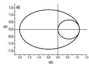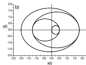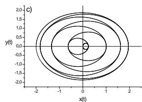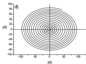 Figure 16: Trajectories obtained both numerically and analytically, a) with $\omega = 0.5\omega_0$ (period two), b) $\omega = 0.75\omega_0$ (period four), c) $\omega = 0.875\omega_0$ (period eight), and d) $\omega = \omega_0$ (resonance, with an aperiodic structure). Let us note that the period doubling sequence generated with the conditions $x_0 = 1$, $f(t) = 0.1\cos(\omega t)$, and $\omega_0 = 1$ is identical to that found in subsection b), with $x_0 = 1$, and $f(t) = 0.1\sin(\omega t)$. We leave the generation of this supplementary cascade as an exercise to the reader. To enable such a simple task, the associated formulas are comprehensively derived and summarized in appendix A. In view of the results of Subsect. a)-c), one may so conclude that period-doubling towards resonance is an intrinsic property of the externally driven harmonic oscillator. Other complex structures obtain by varying the main control parameter $\omega$ while fixing $F$ to any arbitrary value. d) Additional trajectories generated with $f(t) = 0.1 \sin (\omega t), \omega_0 = 1, \text{and} x_0 = 0.$ The corresponding analytical expansions read $$ x (t) = \frac {0 . 1}{1 - \omega^ {2}} (- \omega \sin (t) + \sin (\omega t)) \tag {17a} $$ $$ y (t) = \frac {d x}{d t} = \frac {0 . 1 \omega}{1 - \omega^ {2}} (- \cos (t) + \cos (\omega t)) \tag {17b} $$ The trajectories simulated both numerically and analytically, successively with $\omega = 3\omega_0$ (double loop structure), $\omega = 5\omega_0$ (four loop trajectory), $\omega = 4\omega_0$ (symmetric orbit) and $\omega = 2.5\omega_0$ (asymmetric trajectory) are depicted in Fig. 17.    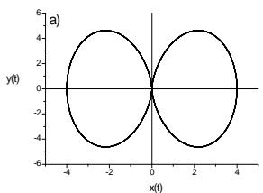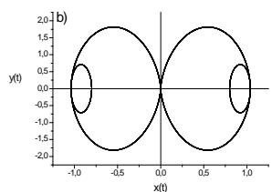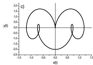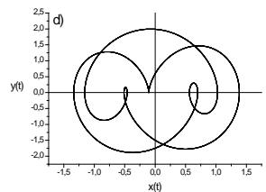 Figure 17: Trajectories obtained both numerically and analytically, successively with a) $\omega = 3\omega_0$, b) $\omega = 5\omega_0$, c) $\omega = 4\omega_0$, and d) $\omega = 2.5\omega_0$. Again, note the commensurate scaling between the driving and the natural frequencies. These examples were arbitrarily chosen amongst countless others. Almost any orbit -with simple or complex structure- may be generated by randomly fixing the system's control parameters and initial conditions. To avoid fuzzy aperiodic trajectories -as that of Fig. 14d- the driving and natural frequencies must scale commensurately. Let us recall that two quantities are commensurable if their ratio is a rational number. If not, these are incommensurable. As a final statement added in proof, let us bring the attention to the fact that an intrinsic nonlinearity carries through the sine or cosine of the external excitation. Consequently, despite its apparent simplicity, the forced harmonic oscillator is a nonlinear system. As such, its behavior has much to share with other nonlinear structures. The originality here is the fact that given the set of initial conditions and the values of the two control parameters, the system's dynamics is fully predictable, through analytical developments of the solutions with a simple relationship, which relates the oscillator movement to the excitation $f(t)$ and to the natural solution $g(t)$, i.e., $x(t) = A(\omega)f(t) + B(\omega)g(t)$. Appendix A summarizes the complete series of solution structures, which connect to the precise initial conditions. These condensate into four formulas that give comprehensive accounts of the predictable dynamics. Let us finally add that if we introduce a third variable, $z = \omega t$, the model transforms into three nonlinearly coupled differential equations of the form $$ \frac {d x}{d t} = y \tag {18a} $$ $$ \frac {d y}{d t} = - \omega_ {0} ^ {2} x + F \cos (z) \tag {18b} $$ $$ \frac {d z}{d t} = \omega \tag {18c} $$ Therefore, it should not be surprising that the model's dynamics carries the same complexities as those of any other nonlinear structure with three degrees of freedom. One non-linear term, i.e., $\cos(z)$, is all it takes to generate a wealth of periodic and aperiodic solutions, with the external frequency as the primary control parameter. The main difference with other nonlinear systems is the depiction of any phase-space trajectory without calling for computer routines, except for the purpose of corroboration and consistency with the analytical formulations. ## VI. CONCLUSION We have revisited the forced-and-undamped harmonic oscillator and disclosed so far overlooked solutions that carry intrinsic nonlinearities. Extensive numerical and analytical examinations give full credit to the outcomes. Despite the complex dynamics these hold, our findings are simple enough to promote their introduction into academic courses in mechanics and vibrations, as well as in mathematics classes that deal with second-order differential equations. The model may serve as a basic example to introduce more complex dynamical systems [12, 15] and familiarize the student with the simple construction of phase space orbits and sequences such as period doubling that were shown to stem from a simple locking phenomenon between the driving frequency and the system's natural frequency. Let us point out the fact that it takes a simple graphical calculator to depict any analytical signal or trajectory. Since the system depends on two control parameters - the amplitude and frequency of the external excitationthat may arbitrarily be selected, the number of solutions, and phase-space trajectories, is theoretically unlimited. Worth insisting on is the construction—unquestionably for the first time in a research and pedagogical paper dedicated to the study of nonlinear dynamical systems—of a series of analytical subharmonic cascades towards resonance. With this respect, our analysis makes clear the fact that period doubling is an intrinsic characteristic that structures systematically and predictably in the case of the forced harmonic oscillator, when the driving and natural frequencies scale commensurately. In addition, next to the unbounded state of resonance, aperiodicity -with bounded trajectories- is the rule whenever the two frequencies scale incommensurately, i.e., when their ratio is a not a rational number. ### APPENDIX A Comprehensive review of the non-autonomous system Let us write the second order differential equation that describes the forced harmonic oscillator when it is driven with an external excitation of the form $$ f (t) = F \sin (\omega t) $$ $$ \frac {d ^ {2} x}{d t ^ {2}} + \omega_ {0} ^ {2} x = F \sin (\omega t) \quad (A 1 a) $$ Considering the free oscillator properties, the general solution reads $$ x (t) = A \sin (\omega_ {0} t) + B \cos (\omega_ {0} t) + C \sin (\omega t) + D \cos (\omega t) \tag {A1b} $$ implying $$ \frac {d ^ {2} x}{d t ^ {2}} = - A \omega_ {0} ^ {2} \sin (\omega_ {0} t) - B \omega_ {0} ^ {2} \cos (\omega t) - C \omega^ {2} \sin (\omega t) - D \omega^ {2} \cos (\omega t) \tag {A1c} $$ So that $$ \left(\omega_ {0} ^ {2} - \omega^ {2}\right) C \sin (\omega t) + \left(\omega_ {0} ^ {2} - \omega^ {2}\right) D \cos (\omega t) = F \sin (\omega t) \tag {A1d} $$ With the solutions $$ D = 0 \tag {A1e} $$ and $$ C = \frac {F}{\omega_ {0} ^ {2} - \omega^ {2}} \tag {A1f} $$ The solution writes $$ x (t) = A \sin (\omega_ {0} t) + B \cos (\omega_ {0} t) + \frac {F}{\omega_ {0} ^ {2} - \omega^ {2}} \sin (\omega t) \tag {A2a} $$ $A$ and $B$ obtain with precise initial conditions. In the case where $\frac{dx}{dt} = 0$, at $t = 0$, we obtain $$ A \omega_ {0} + \frac {F}{\omega_ {0} ^ {2} - \omega^ {2}} \omega = 0 \tag {A2b} $$ i.e., $$ A = - \frac {F}{\omega_ {0} ^ {2} - \omega^ {2}} \frac {\omega}{\omega_ {0}} \tag {A2c} $$ If at $t = 0$, $x(0) = 0$, then $B = 0$, and the solution writes $$ x (t) = \frac {F}{\omega_ {0} ^ {2} - \omega^ {2}} \left(- \frac {\omega}{\omega_ {0}} \sin (\omega_ {0} t) + \sin (\omega t)\right) \tag {A2d} $$ If at $t = 0$, $x = x_0$, then $B = x_0$, and $$ x (t) = \frac {F}{\omega_ {0} ^ {2} - \omega^ {2}} \left(- \frac {\omega}{\omega_ {0}} \sin (\omega_ {0} t) + \sin (\omega t)\right) + x _ {0} \cos (\omega_ {0} t) \tag {A3} $$ If the system is driven with $f(t) = F\cos (\omega t)$, the equation writes $$ \frac {d ^ {2} x}{d t ^ {2}} + \omega_ {0} ^ {2} x = F \cos (\omega t) \tag {A4a} $$ The solution is not quite the same as Eqs (A2d) and (A3). It expands into $$ x (t) = A \cos (\omega_ {0} t) + B \sin (\omega_ {0} t) + C \cos (\omega t) + D \sin (\omega t) \tag {A4b} $$ Which, when plugged into Eq. A(4a) yields $$ \left(\omega_ {0} ^ {2} - \omega^ {2}\right) C \cos (\omega t) + \left(\omega_ {0} ^ {2} - \omega^ {2}\right) D \sin (\omega t) = F \cos (\omega t) \tag {A4c} $$ i.e. $$ D = 0 \tag {A4d} $$ and $$ C = \frac {F}{\omega_ {0} ^ {2} - \omega^ {2}} \tag {A4e} $$ The solution writes $$ x (t) = A \cos \left(\omega_ {0} t\right) + B \sin \left(\omega_ {0} t\right) + \frac {F}{\omega_ {0} ^ {2} - \omega^ {2}} \cos (\omega t) \tag {A5a} $$ If, at $t = 0$, $x = x_0$, then $$ A = x _ {0} - \frac {F}{\omega_ {0} ^ {2} - \omega^ {2}} \tag {A5b} $$ We determine $B$ with $dx / dt = 0$, at $t = 0$ $$ \frac {d x}{d t} = - A \omega_ {0} \sin (\omega_ {0} t) + B \omega_ {0} \cos (\omega_ {0} t) - C \omega \quad \sin (\omega t) + D \omega \quad \cos (\omega_ {0} t) = 0 \tag {A5c} $$ From which we extract, $B = D = 0$, and $$ x (t) = \left(x _ {0} - \frac {F}{\omega_ {0} ^ {2} - \omega^ {2}}\right) \cos (\omega_ {0} t) + \frac {F}{\omega_ {0} ^ {2} - \omega^ {2}} \cos (\omega t) \tag {A5d} $$ i.e. $$ x (t) = \frac {F}{\omega_ {0} ^ {2} - \omega^ {2}} \left(- \cos (\omega_ {0} t) + \cos (\omega t)\right) + x _ {0} \cos (\omega_ {0} t) \tag {A5e} $$ The case corresponding to $x(0) = 0$ is considered in the text. See Eq. (8a) or Eq. (A7c). Solution at resonance For $\omega = \omega_{o}$, Eq. (A4a) writes $$ \frac {d ^ {2} x}{d t ^ {2}} + \omega_ {0} ^ {2} x = F \cos \left(\omega_ {0} t\right) \tag {A6a} $$ Since we know that at resonance the amplitude grows indefinitely, we try the following solution $$ x (t) = A t \sin \left(\omega_ {0} t\right) + B t \cos \left(\omega_ {0} t\right) \tag {A6b} $$ Transforming Eq. (A6a) into $$ 2 \omega_ {0} A \cos (\omega_ {0} t) - 2 \omega_ {0} B \sin (\omega_ {0} t) = F \cos (\omega_ {0} t) \tag {A6c} $$ i.e. $$ B = 0 \quad (\mathrm {A} 6 \mathrm {d}) $$ and $$ A = \frac {F}{2 \omega_ {0}} \tag {A6e} $$ The general solution expands into $$ x (t) = c _ {1} \sin \left(\omega_ {0} t\right) + c _ {2} \cos \left(\omega_ {0} t\right) + \frac {F}{2 \omega_ {0}} t \cos \left(\omega_ {0} t\right) \tag {A6f} $$ With the initial conditions $x(0) = 0$ and $dx/dt = 0$, we are left with $$ x (t) = - \frac {F}{2 \omega_ {0} ^ {2}} \sin (\omega_ {0} t) + \frac {F}{2 \omega_ {0}} t \cos (\omega_ {0} t) \tag {A6g} $$ For large $t$ 's, the first term becomes negligible, and $$ x (t) = \frac {F}{2 \omega_ {0}} t \cos \left(\omega_ {0} t\right) \tag {A6h} $$ Indicative of linearly growing amplitudes, conforming to the graph of Fig. 3. Summary of the solutions For straightforward comparisons between the formulas -and forthright signal and orbit depictions- let us summarize the solutions. ### a) $f(t) = F\sin (\omega t),x(0) = 0$ $$ x (t) = \frac {F}{\omega_ {0} ^ {2} - \omega^ {2}} \left(- \frac {\omega}{\omega_ {0}} \sin (\omega_ {0} t) + \sin (\omega t)\right) \tag {A7a} $$ ### b) $f(t) = F\sin (\omega t),x(0) = x_0$ $$ x (t) = \frac {F}{\omega_ {0} ^ {2} - \omega^ {2}} \left(- \frac {\omega}{\omega_ {0}} \sin (\omega_ {0} t) + \sin (\omega t)\right) + x _ {0} \cos (\omega_ {0} t) \tag {A7b} $$ ### c) $f(t) = F\cos (\omega t),x(0) = 0$ $$ x (t) = \frac {F}{\omega_ {0} ^ {2} - \omega^ {2}} \left(- \cos \left(\omega_ {0} t\right) + \cos (\omega t)\right) \tag {A7c} $$ ### d) $f(t) = F\cos (\omega t),x(0) = x_0$ $$ x (t) = \frac {F}{\omega_ {0} ^ {2} - \omega^ {2}} (- \cos (\omega_ {0} t) + \cos (\omega t)) + x _ {0} \cos (\omega_ {0} t) \tag {A7d} $$ As fully demonstrated in the text, through the subharmonic sequences, even though only slight differences appear between the four expressions, each formula carries distinctive dynamics. Again, let us insist on the fact that, whatever the initial conditions, all four formulas bear the form $x(t) = A(\omega)f(t) + B(\omega)g(t)$. An indication of the nonlinear dependence of the oscillator displacement with respect to the external excitation. Indeed, if we represent $x(t)$ vs $f(t)$, we recover a linear segment in the case of a linear response (Fig.A1-a) and a nonlinear curve in the case of nonlinear response (Fig.A1-b). Both curves correspond to $F = 1$, $\omega_0 = 1$, and $\omega = 2\omega_0$.  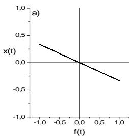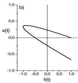 Figure A1: Response $x(t)$ vs excitation $f(t)$, in the case of a) a linear solution, and b) a nonlinear solution. #### APPENDIX B Useful trigonometry To understand the modulation effect that occurs in the presence of the driving and the natural frequencies, it is useful to establish the following relationship $$ \cos \left(\omega_ {0} t\right) - \cos (\omega t) = 2 \sin \left(\frac {\omega + \omega_ {0}}{2} t\right) \sin \left(\frac {\omega - \omega_ {0}}{2} t\right) \tag {B1a} $$ Let us start with $$ \cos (\omega t) = \cos \left(\frac {\omega + \omega_ {0}}{2} t + \frac {\omega - \omega_ {0}}{2} t\right) \tag {B1b} $$ which transforms into $$ \cos (\omega t) = \cos \left(\frac {\omega + \omega_ {0}}{2} t\right) \cos \left(\frac {\omega - \omega_ {0}}{2} t\right) - \sin \left(\frac {\omega + \omega_ {0}}{2} t\right) \sin \left(\frac {\omega - \omega_ {0}}{2} t\right) \tag {B1c} $$ Furthermore $$ \cos \left(\omega_ {0} t\right) = \cos \left(\frac {\omega + \omega_ {0}}{2} t - \frac {\omega - \omega_ {0}}{2} t\right) \tag {B1d} $$ converts into $$ \cos \left(\omega_ {0} t\right) = \cos \left(\frac {\omega + \omega_ {0}}{2} t\right) \cos \left(\frac {\omega - \omega_ {0}}{2} t\right) + \sin \left(\frac {\omega + \omega_ {0}}{2} t\right) \sin \left(\frac {\omega - \omega_ {0}}{2} t\right) \tag {B1e} $$ $$ - \cos (\omega_ {0} t) + \cos (\omega t) = - 2 \sin \left(\frac {\omega + \omega_ {0}}{2} t\right) \sin \left(\frac {\omega - \omega_ {0}}{2} t\right) \tag {B1f} $$ and $$ x (t) = \frac {F}{\omega_ {0} ^ {2} - \omega^ {2}} \left(- \cos \left(\omega_ {0} t\right) + \cos (\omega t)\right) = - \frac {2 F}{\omega_ {0} ^ {2} - \omega^ {2}} \sin \left(\frac {\omega + \omega_ {0}}{2} t\right) \sin \left(\frac {\omega - \omega_ {0}}{2} t\right) \tag {B1g} $$ This last relation indicates that in the presence of the driving and natural solutions, the signal outputs in the form of a high frequency component $f + f_{0}$ modulated by a lower frequency at $f - f_{0}$, an example of which is represented in Fig. 9a of the text. Also note that the amplitude of the displacement is twice that obtained when the natural solution is neglected (compare Eq. (B1g) and Eq. (4h) of the text). This means that the resonant phenomenon becomes more important when the free oscillator frequency is included. Consequently, added to the butterfly effect, which transforms regular signals into turbulent ones whenever the driving and natural frequencies scale incommensurately, catastrophes -as those described in the text- are (were) more likely to occur! #### APPENDIX C Note added in proof Let us rewrite Eqs (6) $$ \frac {d x}{d t} = y \tag {C1a} $$ $$ \frac {d y}{d t} = - \omega_ {0} ^ {2} x + F \cos (\omega t) \tag {C1b} $$ And define a new variable $$ z = \omega t \tag {C2a} $$ So that $$ \frac {d z}{d t} = \omega \tag {C2b} $$ Eqs (C1) rewrite in the form $$ \frac {d x}{d t} = y \tag {C3a} $$ $$ \frac {d y}{d t} = - \omega_ {0} ^ {2} x + F \cos (z) \tag {C3b} $$ $$ \frac {d z}{d t} = \omega \tag {C3c} $$ We are in the presence of a three-dimensional system nonlinearly coupled through the term $\cos (z)$. Therefore, it should be of no surprise to retrieve typical properties of other nonlinearly coupled differential equations as fully described in the text [12].

Generating HTML Viewer...

References

14 Cites in Article
H Haken (1975). Analogy between higher instabilities in fluids and lasers.
Edward Lorenz (1963). Deterministic Nonperiodic Flow.
R Feynman,R Leighton,M Sands (2014). Exercises for The Feynman Lectures on Physics.
G Adomian,R Rach (1994). A new algorithm for solution of the harmonic oscillator by decomposition.
Grant Fowles,George Cassiday,R Robinett (1986). <i>Analytical Mechanics, 6th ed.</i>.
Sabih Hayek (2003). Mechanical Vibration and Damping.
No ethics committee approval was required for this article type.
Data Availability
Not applicable for this article.
How to Cite This Article
Belkacem Meziane. 2026. \u201cThe Harmonic Oscillator, Complex-Dynamics Predictability, and the Beauty of Trigonometry: Subharmonic Cascades towards Resonance\u201d. Global Journal of Research in Engineering - J: General Engineering GJRE-J Volume 23 (GJRE Volume 23 Issue J2).
Explore published articles in an immersive Augmented Reality environment. Our platform converts research papers into interactive 3D books, allowing readers to view and interact with content using AR and VR compatible devices.
Your published article is automatically converted into a realistic 3D book. Flip through pages and read research papers in a more engaging and interactive format.
Our website is actively being updated, and changes may occur frequently. Please clear your browser cache if needed. For feedback or error reporting, please email [email protected]
Thank you for connecting with us. We will respond to you shortly.