## I. INTRODUCTION The problem of the moving black-body radiation arose in^1907 - almost immediately after the creation of Special relativity (SR). It is in this year that Kurt von Mosengeil's big article was published in der Annalen der Physik [1]. This work supervised by Max Planck underlies his relativistic thermodynamics [2]. The great scientist considered the theory of the black-body radiation to be well-studied and the most suitable for formulating foundations of thermodynamics correct over the entire whole interval of object velocities v, i.e., ranging from zero to the velocity of light in vacuo. In article [1] a system is studied comprising a radiator of electromagnetic waves, receiver and reflector (mirror). The radiators are receivers at the same time. The three elements are moving uniformly and rectilinearly in space with a relativistic velocity forming an acute angle with one another. As a result, the temperature transformation law was obtained under relativistic conditions: $$ T = T _ {0} \sqrt {1 - \beta^ {2}}, \tag {1} $$ where $T_0$ is the temperature if $\nu < c$ (here and below index "0" means that the given quantity concerns normal conditions); $\beta = \nu / c$. For more than 50 years formula (1) had not been called in question until X.Ott's article was published [3], in which the relativistic temperature was shown to transform following another law: $$ T = T _ {0} / \sqrt {1 - \beta^ {2}}. \tag {2} $$ The expression (2) was obtained by X.Ott for a variety of physical processes including electromagnetic radiation. However unlike Mosengeil, X.Ott elected another approach for studying the process of electromagnetic wave radiation under relativistic conditions. He examined wave emission of individual atoms, whereas Mosengeil studied black-body radiation, as we have noticed above. In particular, in [1] Stefan-Boltzmann's law was obtained: $$ \varepsilon_ {0} = \frac {E _ {0}}{V _ {0}} = a T _ {0} ^ {4}, \tag {3} $$ based on the famous Planck formula derived first semiempirically: $$ \rho(\omega,T)\,d\omega = \frac{8\pi h\omega^3\,d\omega}{c^3\left(e^{\frac{h\omega}{kT}} - 1\right)} $$ where $E_0$ is the radiation energy of the black-body; $V_0$ is the volume; $a$ is Stephan-Boltzmann's constant (J/cc·grad $^4$ ); $\rho(\omega, T)$ is the radiative energy density (J/cc); $k$ is Boltzmann's constant; $\omega$ is the frequency of oscillator radiation. As known, Stefan-Boltzmann's constant equals: $$ a = \frac {k ^ {4} \pi^ {2}}{1 5 h ^ {3} c ^ {3}}. \tag {5} $$ X.Ott's article has induced a long-term polemic on the temperature transformation under relativistic conditions. Some researchers adhered to Planck-Einstein's viewpoint; the others adhered to X.Ott's. Some scientists considered the temperature to be a relativistic invariant [4]. There appear absolutely exotic opinions. For example, the authors of Ref. [5] arrived at a conclusion of the temperature under relativistic conditions being changed both according to Planck, and to Ott, and to Callen and Horwitz as the able situation requires. Moreover, P. Landsberg and G. Matsas have decided to put end to the long-time dispute [6, 7]. In particular, they write (I cite): "...the proper temperature T alone is left as the only temperature of universal significance. This seems to complete a story started 90 years ago \[8\](more than^100 years today - E.V.) of how usual temperature transforms, and to conclude a controversy [3] of 33 years' standing". (50 years' today). What is authors' opinion [6, 7] based on? Their basis is as follows. First of all, the authors used an Unruh-De Witt detector, i.e., a two-level monopole, with a unit interval of the radiation energy $\hbar \omega^{\prime}$. Then the authors [6, 7] suppose that black-body radiation with the proper temperature $T$ is at rest in some inertial reference frame $S$. The excitation rate of the detector moving with a constant velocity $\nu$ is found from quantum field theory. It is proportional to the particle number density $n^{\prime}(\omega^{\prime}, T, \nu)d\omega^{\prime}$. As a result, the following formula was obtained: $$ n^\prime\left(\omega^\prime,T,v\right)d\omega^\prime=\frac{\omega^\prime kT\sqrt{1-v^{2}/c^{2}}}{4\pi^{2}c^{2}v\hbar}\ln\left(\frac{1-e^{-\left(\hbar\omega^\prime\sqrt{1-v/c}\right)/kT\sqrt{1-v/c}}}{1-e^{-\left(\hbar\omega^\prime\sqrt{1-v/c}\right)/kT\sqrt{1+v/c}}}\right)d\omega^\prime, $$ which, as the authors of [6, 7] noted, could not be reduced at $v = 0$ to the well-known formula $$ n ^ {\prime} \left(\omega^ {\prime}, T ^ {\prime}, v\right) d \omega^ {\prime} = \frac{\omega^ {2} / c ^ {3}}{2 \pi^ {2} \left(e ^ {\hbar \omega^ {\prime} / k T ^ {\prime}} - 1\right)} d \omega^ {\prime}. $$ We obtain from (6) an expression which does not defy interpretation, as $\nu \rightarrow c$. In opinion of P. Lands berg and G. Matsas, formula (6) is absolutely correct, thus it is unnecessary to speak about an unified law of temperature transformation under relativistic conditions. However it is not completely the case. Both the results obtained by Mosengeil (and soon used by Planck), and the mathematical monster (6) are incorrect. It is necessary to admit that the main reason of such a dramatic situation with a relativistic temperature is a giant scientific authority of Max Planck first and Albert Einstein. Naturally, after publishing X.Ott's article this work was carefully checked. Errors had not been found. But nobody dared check the works [1, 2, 8]. These articles were carried out just after the creation of Special Relativity (SR) when nobody had known on the Bose-Einstein distribution. As we have noticed above, Planck's well-known formula, concerning black-body radiation, was obtained by a semiempirical way without involving this distribution. After the discovery of this distribution, in the twenties of last century, Planck's formula was already obtained with its help. However if the radiator of electromagnetic waves is moving with a relativistic velocity, the form of Bose-Einstein distribution changes drastically – it becomes at least a function of two variables, which immediately follows from SR electrodynamics. 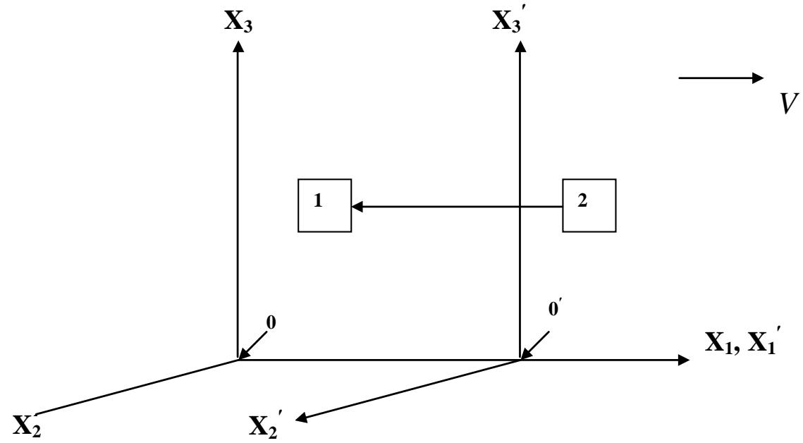 Fig.1: $X_{1}, X_{2}, X_{3}$ and $X_{1}^{\prime}, X_{2}^{\prime}, X_{3}^{\prime}$ are the laboratory reference frame and that moving uniformly and rectilinearly with the velocity v. 1 is the observer at rest; 2 is the radiating black body Indeed, examine the simplest case represented in the Fig.1. As seen, there are two reference frames. One of them (with primes) is moving uniformly and rectilinearly with the velocity $\mathbf{v}$. There is a cylindrical object at rest in the moving reference frame. There is a cylindrical cavity in the object. The walls of the cavity are a black-body. They are emitting and absorbing photons. There is a very small hole on a face-wall of the object (see Fig.1). The flux of photons is flowing out the cavity. Since the hole is very small, the equilibrium of the photon gas in the cavity does not disturb practically. The photon radiator is at rest in the moving reference frame. An observer is at rest in the laboratory reference one. The observer is detecting photons (the energy of the electromagnetic wave). Here Maxwell's 3-D tensor of energy-momentum $\sigma_{\alpha \beta}$ has only one component - $\sigma_{11}$. It is equal to the density of energy in the wave [9]. Knowing the density of energy in the flux of photons, we can estimate the density of energy of the photon gas in the cavity in practice. If the angle $\theta$ between $\mathbf{v}$ and the observer is $3\pi /2$ (the object is moving away from the observer), then the radiation frequency of the oscillator $\omega$ will be for this case equal to $$ \omega = \omega_ {0} \frac {\sqrt {1 - \beta^ {2}}}{1 + \beta}. \tag {8a} $$ If the object is moving to the observer i.e., the velocity of the system is equal to $-\mathbf{v}$, then $$ \omega = \omega_{0} \frac{\sqrt{1 - \beta^{2}}}{1 - \beta}. $$ Denote the frequencies $\omega$ in (8a) and (8b) as $\omega_{1}$ and $\omega_{2}$ then $$ \overline {{\omega}} = \frac {\omega_ {1} + \omega_ {2}}{2} = \frac {\omega_ {0}}{\sqrt {1 - \beta^ {2}}}, \tag {8c} $$ If the angle $\theta$ were $(- \pi / 2)$, then the formula for the frequency transformation would have another form, namely: $$ \omega = \omega_ {0} \sqrt {1 - \beta^ {2}}. \tag {9} $$ for the observer in the laboratory reference frame. Thus without taking into consideration (8) and (9), we cannot evidently use the well-known Bose-Einstein distribution for obtaining the Stefan-Boltzmann law when the object under study is moving with relativistic speed. The aforesaid allows us to formulate a main goal of our work - obtaining a radiation law for the black-body moving with a relativistic velocity when the angle $\theta$ between the moving velocity $\mathbf{v}$ and the observer is $3\pi / 2$ (see Fig.1). A solution of the problem will be performed by the methods given in [9]. Here we must be added the following. Attempts have been made to obtain the law connecting the radiation intensity with the temperature when relativistic effects are involved [10, 11]. For example, in [11] an ultrarelativistic plasma is examined containing electrons and positrons. Their annihilation generates electromagnetic radiation. Its intensity is defined, in particular, with the help of a one-dimensional Bose-Einstein distribution. It is proportional to the plasma temperature to the fourth power, with the velocity of the object as a whole being equal to zero. It is plasma particles that are in motion. ## II. METHODS AND RESULTS ### a) Definition of the number of field oscillators with a given frequency when the angle $\theta$ is $3\pi /2$ (Fig.1) Assume that we have an opaque object with an inner cylindrical cavity. Its surface is a black body heated up to some temperature $T$. There is a thermodynamical equilibrium in the cavity between its inner surface and electromagnetic radiation. There is a very small hole in the object cover, through which electromagnetic waves radiate out of the cavity (see Fig.1). The object is moving uniformly and rectilinear with the velocity $\mathbf{v}$ together with the reference frame. The radiation from the cavity is detected with a device being at rest in a laboratory reference frame. First of all, we will show that the Stefan-Boltzmann law (3) is incorrect over the whole range of object motion velocities, i.e., from zero up to $v \rightarrow c$. Indeed, according to X. Ott [3], the radiation energy in the cavity is equal to: $$ E = \frac {\sum_ {1} ^ {n} h \omega_ {0} ^ {(n)}}{\sqrt {1 - \beta^ {2}}}, n = 1, 2, \dots I, \tag {10} $$ then the electromagnetic energy density $$ \varepsilon = \frac{E _ {0}}{V _ {0} \left(1 - \beta^ {2}\right)} = \frac{\sum_ {1} ^ {n} h \omega_ {0} ^ {(n)}}{V _ {0} \left(1 - \beta^ {2}\right)}, \, n = 1, 2, \dots , \tag{11} $$ where $n$ is an oscillator serial number, $\omega^{(n)}$ is the frequency of its oscillations. For the flux of photons moving away from the cavity (see Fig1), the equations (10) and (11) are also correct. Indeed, there is only one component $\sigma_{11}$ of Maxwell's stress tensor (see above). The component is equal $$ \begin{array}{l} \sigma_ {1 1} \sim E _ {2} ^ {2} + E _ {3} ^ {2} + H _ {2} ^ {2} + H _ {3} ^ {2} = \frac {E _ {0 2} ^ {2} + E _ {0 3} ^ {2} + H _ {0 2} ^ {2} + H _ {0 3} ^ {2}}{1 - \beta^ {2}}, \\E _ {2 (3)} = \frac {E _ {0 2 (0 3)}}{\sqrt {1 - \beta^ {2}}}; H _ {2 (3)} = \frac {H _ {0 2 (0 3)}}{\sqrt {1 - \beta^ {2}}} \\\end{array} $$ where $E_{2(3)}, E_{02(03)}$ are the intensity components of the electric field in the directions 2 and 3 for the observers in the laboratory reference frame and for the observer moving with the system under study correspondingly; $H_{2(3)}, H_{02(03)}$ are the intensity components of the magnetic field in the directions 2 and 3 for the above observers. No matter how the temperature of the system transforms, i.e., according to Planck or to Ott or to Callen and Horwitz, we shall always arrive at the point of absurdity. Indeed, let the temperature transform, e.g., according to Planck, i.e., to (1). In this case the right side of (3) will have the following form $a T_0^4 \left( 1 - \beta^2 \right)^2$. Then, as seen from (11), the right side of (3) appears to tend to zero as $v \to c$, while the left side of this formula to increase infinitely. This indicates a close connection between the radiation law of a moving black body and the temperature transformation under relativistic conditions. Now find the number of oscillators $g(\omega_1, \omega_2) = d\omega_1 d\omega_2$ with frequencies in intervals $\omega_1, \omega_1 + d\omega_1$ and $\omega_2, \omega_2 + d\omega_2$ and a given polarization in the cavity using the well-known procedure [9]. The following fact should be pointed out at once. The number of these oscillators is a function of two variables. The reason for that was explained above but here the following should be noted. If a spherical coordinate system is used for the case $\nu < c$, then in our case it is convenient to use a cylindrical one taking account of formulae (8) and (9). The classical approach to finding the quantity $g(\omega)d\omega$ is based on using the number space $n$ followed by transition to a spherical space of the wave vector $k = |k| = n\frac{2\pi}{L}$, where $L$ is the normalized cube edge, and finally to the spherical space of frequencies $\omega$. In the case studied we use a cylindrical space representable as two spaces - flat circular and linear perpendicular to one another. Then to define the necessary quantity we shall use two coordinate systems: polar and one-dimensional Euclidean, i.e., a straight line. The amount of numbers within the spherical layer $dn$ of the spherical space is $4\pi n^2 dn$ \[9\](the spherical coordinate system). The amount of numbers $n_1$ in the circular layer is equal to $2\pi n_1 dn_1$ (the polar coordinate system). As to $n_2$ in a linear interval of one-dimension space, it will be equal to $dn_2$. As a result, we have for the whole system: $$ g \left(\omega_ {1}, \omega_ {2}\right) d \omega_ {1} d \omega_ {2} = 2 \pi n _ {1} d n _ {1} d n _ {2}. \tag {12} $$ Turning from a number space to a wave vector space and finally to a frequency one, we shall have: $$ \begin{array}{l} g \left(\omega_ {1}, \omega_ {2}\right) d \omega_ {1} d \omega_ {2} = 2 \pi m _ {1} d n _ {1} d n _ {2} = \frac {2 \pi k _ {1} d k _ {1} d k _ {2}}{(2 \pi) ^ {3}} \Delta L _ {1} ^ {2} \Delta L _ {2} = \frac {\omega_ {1} d \omega_ {1} d \omega_ {2}}{(2 \pi) ^ {2} c ^ {3}} \Delta L _ {1} ^ {2} \Delta L _ {2} = \\= \frac {\omega_ {1} d \omega_ {1} d \omega_ {2}}{(2 \pi) ^ {2} c ^ {3}} \Delta V. \tag {13} \\\end{array} $$ In case of electromagnetic waves should be taken into account two polarizations, and then we shall have: $$ g\left(\omega_ {1}, \omega_ {2}\right) d \omega_ {1} d \omega_ {2} = \frac{\omega_ {1} d \omega_ {1} d \omega_ {2}}{2 \pi^ {2} c ^ {3}} \Delta V.\tag{14} $$ Here it is important to emphasize that formula (14) is correct for the observer at rest in a real space monitoring, from the referring frame, the object moving then uniformly and rectilinearly with the relativistic velocity $\mathbf{v}$. Since the radiation is thermal the average volume of the oscillators with a given polarization will almost be independent of time. In this case, it is unnecessary to define oscillator numbers in Minkowski space. ### b) Relativistic temperature as either a vector or a tensor Now we should make a new attempt to solve some problems connected with the relativistic temperature. First of all, we should clarify if this thermodynamic parameter is a scalar or appears to be a vector or a tensor. In this connection we should first recall the formulae for velocity addition in SR. As known, the components of the total velocity in the directions $X_{2}$ or $X_{3}$ will tend to zero for the observer in the laboratory reference frame as $v \rightarrow c$ (see Fig.1). In turn, the component parallel to axes the $X_{1}$ will not do that. This suggests immediately that the temperature becomes a mathematical object different from a scalar. What is the object? Until very recently the temperature in the above case is considered to be either a scalar or a quantity forming a vector with other quantities. For example, in [10] V. Hamity represents this thermodynamical parameter as $$ \Theta^\mu = \frac{v^\mu}{\hat{T}}, \quad \mu = 0,1,2,3, $$ where $\nu^{\mu}$ is a unit 4-vector in Minkowski space, moreover $$ v ^ {\mu} = \left[ v ^ {0}, v ^ {\alpha} \right], \alpha = 1, 2, 3, \tag {16} $$ i.e., $\pmb{\nu}^{\alpha}\equiv \mathbf{v}$ is a velocity vector in Euclidean space; $$ v ^ {\mu} v _ {\mu} = 1. \tag {17} $$ Further, developing the idea of temperature vector representation, the author of [10] finally comes to the following expression: $$ \beta_ {\mu} = v _ {\mu} / k T, \tag {18} $$ with $\beta_{\mu} = (\beta, 0,0,0)$, then $$ \beta_{\mu} = \delta_{\mu}^{0} / kT, \quad \delta_{\mu}^{\nu} = \left( \begin{array}{c c c c} 1 & 0 & 0 & 0 \\0 & 1 & 0 & 0 \\0 & 0 & 1 & 0 \\0 & 0 & 0 & 1 \end{array} \right). $$ Other authors, e.g., [12], also tried to represent the relativistic temperature exclusively as a vector. However, in our opinion, this approach to the problem is incorrect, since the photon gas in the cavity is a continuous medium. Then an expanded tensor approach is necessary to describe energy processes in it. In this case the second thermodynamics law can be represented in Minkowski space as $$ \delta\sigma=\frac{\delta Q^{ijk}g_{jk}}{T^{i\alpha\beta}g_{\alpha\beta}};i,j,k=1,2,3,4;\alpha,\beta=1,2,3,4, $$ where the heat $Q$ and the temperature $T$ are tensors of rank 3, but $\pmb{g}_{jk},\pmb{g}_{\alpha \beta}$ are covariant fundamental tensors. Formula (20) needs a special explanation. As known, M.Planck assumed that $\sigma \neq \sigma (\mathbf{v})$, i.e., the entropy of the system varies exclusively owing to thermodynamical processes in the object under study and is independent of its velocity relative to the observer in the laboratory reference frame [2]. As will be shown below, the law (20) agrees with the Planck statement. Further, the contraction of the heat and temperature tensors with the fundamental tensors transforms them to the vectors multiplied into scalar quantities. The latter are invariant parts of the above tensors that do not vary when passing from one reference frame to another. As to the vectors, their components are equal to unity when the moving system 4-velocity equals to zero, i.e., $$ n = \left( \begin{array}{l} 1 \\1 \\1 \\i \end{array} \right), \tag {21} $$ $$ n ^ {1} = \frac {n ^ {1} - \beta n ^ {4}}{\sqrt {1 - \beta^ {2}}}, n ^ {2} = n ^ {2}, n ^ {3} = n ^ {3}, n ^ {4} = \frac {- \beta n ^ {1} + n ^ {4}}{\sqrt {1 - \beta^ {2}}}, \tag {22} $$ where $i$ is imaginary unit; $\beta = \nu /c$ Then the contraction in (20) of two vector quantities in indices $i$ gives a scalar quantity, which is invariant under the Lorentz transformations. As to heat and the temperature, their invariant parts vary exclusively owing to purely thermodynamic reasons. In turn, the vector components vary exclusively, when passing from one reference frame to another. In both cases either the heat or the temperature are inversely proportional to the quantity $\sqrt{1 - \beta^2}$. Then the entropy will not change in the absence of heat input into the system. The latter is in a full accord with the results obtained in works [13, 14, and 15] where the temperature was shown to transform under relativistic conditions in inverse proportion to the quantity $\sqrt{1 - \beta^2}$. Then we can represent the temperature in Minkowski space as $$ T^{i} = T^{i\alpha\beta} g_{\alpha\beta} = \mathrm{T} n^{i} = \mathrm{T} n, $$ where $\mathbf{T}$ is the invariant part of the tensor magnitude of rank 3, i.e., $T^{i\alpha \beta}$. In the real space formulae (20) and (23) remain unchanged with the only difference that, first, we now use affine tensors, second, the dependences (21) and (22) take the form: $$ \mathsf{n} = \left( \begin{array}{l} 1 \\1 \\1 \end{array} \right), \tag{24} $$ $$ n^{1} = \frac{n^{1}}{\sqrt{1 - \beta^{2}}}, n^{2} = n^{2}, n^{3} = n^{3}. $$ At $\nu = 0$ the spatial components of $T^i$ coincide in Euclidean space with the same components in Minkowski space. In space-time the components of squared sum of the vector quantity $\mathbf{T}\mathbf{n}$ read $$ \mathrm {T} ^ {2} n _ {x} ^ {2} + \mathrm {T} ^ {2} n _ {y} ^ {2} + \mathrm {T} ^ {2} n _ {z} ^ {2} = \mathrm {T} ^ {2} n _ {\tau} ^ {2} = \mathrm {T} _ {x} ^ {2} + \mathrm {T} _ {y} ^ {2} + \mathrm {T} _ {z} ^ {2} = \mathrm {T} _ {\tau} ^ {2}, \tag {26} $$ invariant in all inertial reference frames. On the other hand the invariant of this sort gives in Euclidean space $$ \mathrm{T}^{2}n^{\prime 1}n_{1}^\prime + \mathrm{T}^{2}n^{\prime 2}n_{2}^\prime + \mathrm{T}^{2}n^{\prime 3}n_{3}^\prime = \mathrm{T}^{2}n^{1}n_{1} + \mathrm{T}^{2}n^{2}n_{2} + \mathrm{T}^{2}n^{3}n_{3} = \mathrm{T}_{x}^{2} + \mathrm{T}_{y}^{2} + \mathrm{T}_{z}^{2} = \mathrm{invar}, $$ taking into consideration that $n_1' n' = 1$ (affine tensors), i.e., the spatial part of the invariant connected with the temperature 4-tensor is completely identical to the invariant connected with the temperature 3-tensor. It is very important since it allows one to solve our problem directly in Euclidean space. As to the ultrarelativistic plasma considered in [11], the aforesaid will be valid in this case as well, which will be discussed below. ### c) Radiation Intensity Dependence vs. Temperature for a Moving Black Body Consider a black body moving uniformly and rectilinearly at angle $\theta = 3\pi /2$ with respect to the observer in the laboratory reference frame. Based on the aforesaid and on classical methods (i.e., for $\nu < c$, see, e.g., [9, 16]) we can now begin its solution taking into consideration the follow. Now we use a cylindrical coordinate system and certain elementary normalizing volume in it. This volume contains two independent oscillators. The first oscillator is oriented parallel to axis 1. The second one is oriented perpendicularly to this axis. Then we can write an expression for the average total energy $\bar{\varepsilon}$ of the linear oscillators with quantum numbers $n_1 = n_2 = 1$ as follows (cylindrical space, zero oscillations are neglected): $$ \bar{\varepsilon} = \left(\varepsilon_{1} + \varepsilon_{2}\right)^{n_{1}, n_{2} = 1} = \frac{\hbar \left(\omega_{1} + \omega_{2}\right)}{\left(e^{\frac{\hbar \omega_{1}}{\theta_{1}}} - 1\right) \left(e^{\frac{\hbar \omega_{2}}{\theta_{2}}} - 1\right)} $$ where $\omega_{1}$ and $\omega_{2}$ are the frequencies of oscillators in the direction perpendicular and parallel to the velocity of the moving object; $n_{1}$ and $n_{2}$ are positive (quantum) integers for the oscillators in the first and second directions. In this case $n_{1} = n_{2} = 1$, since photons are bosons, they can be in one quantum state; $T_{1}, T_{2}$ are the values of the temperature tensor components. Obtaining the formula (28), we have used the law of the probability multiplying since the both oscillators are independent one another. Then the average volume of the total energy $\varepsilon$ of the electromagnetic field per unit volume in the moving cavity proves to equal $$ \bar{\varepsilon} = \frac{E_{0}}{V_{0} \left(1 - \beta^{2}\right)} = \frac{2 \hbar}{\left(2 \pi\right)^{2} c^{3}} \int_{0}^{\infty} \frac{\omega_{1}^{2} d\omega_{1}}{\left(e^{\frac{\hbar \omega_{1}}{\theta_{1}}} - 1\right)} \int_{0}^{\infty} \frac{d\omega_{2}}{\left(e^{\frac{\hbar \omega_{2}}{\theta_{2}}} - 1\right)} + \frac{2 \hbar}{\left(2 \pi\right)^{2} c^{3}} \int_{0}^{\infty} \frac{\omega_{1} d\omega_{1}}{\left(e^{\frac{\hbar \omega_{1}}{\theta_{1}}} - 1\right)} \int_{0}^{\infty} \frac{\omega_{2} d\omega_{2}}{\left(e^{\frac{\hbar \omega_{2}}{\theta_{2}}} - 1\right)}. \tag{29} $$ As a result, we have obtained, in fact, four improper integrals, three of them converge. The last two integrals in (29) differ only by variables. They are easily calculated using variable transformations as follows: $$ y _ {1 (2)} = \frac {\hbar \omega_ {1 (2)}}{\theta_ {1 (2)}} = \frac {\hbar \omega_ {1 (2)}}{k T _ {1 (2)}}, \tag {30} $$ $$ I _ {1} = \frac{2 \hbar}{(2 \pi) ^ {2} c ^ {3}} \int_ {0} ^ {\infty} \frac{\omega_ {1} d \omega_ {1}}{\left(e ^ {\frac{\hbar \omega_ {1}}{\theta_ {1}}} - 1\right) ^ {0}} \int_ {0} ^ {\infty} \frac{\omega_ {2} d \omega_ {2}}{\left(e ^ {\frac{\hbar \omega_ {2}}{\theta_ {2}}} - 1\right)} = \frac{2 \theta_ {1} ^ {2} \theta_ {2} ^ {2}}{(2 \pi) ^ {2} \hbar^ {3} c ^ {3}} \int_ {0} ^ {\infty} \frac{y _ {1} d y _ {1}}{\left(e ^ {y _ {1}} - 1\right) ^ {0}} \int_ {0} ^ {\infty} \frac{y _ {2} d y _ {2}}{\left(e ^ {y _ {2}} - 1\right)} = \\= \frac{2 \theta_ {1} ^ {2} \theta_ {2} ^ {2}}{\left(2 \pi\right) ^ {2} \hbar^ {3} c ^ {3}} \cdot \frac{\pi^ {4}}{3 6} = \frac{k ^ {4} \pi^ {2} T _ {1} ^ {2} T _ {2} ^ {2}}{7 2 \hbar^ {3} c ^ {3}} = 0.2 0 8 a T _ {1} ^ {2} T _ {2} ^ {2}, \tag{31} \end{array} $$ where $a$ is the Stefan-Boltzmann constant, i.e., $$ a = \frac {k ^ {4} \pi^ {2}}{1 5 \hbar^ {3} c ^ {3}}. \tag {32} $$ $$ I _ {2} = \frac{2 \hbar}{(2 \pi) ^ {2} c ^ {3}} \int_ {0} ^ {\infty} \frac{\omega_ {1} ^ {2} d \omega_ {1}}{\left(e ^ {\frac{\hbar \omega_ {1}}{\theta_ {1}}} - 1\right)} \int_ {0} ^ {\infty} \frac{d \omega_ {2}}{\left(e ^ {\frac{\hbar \omega_ {2}}{\theta_ {2}}} - 1\right)} = \frac{2 \hbar}{(2 \pi) ^ {2} c ^ {3}} I _ {2} ^ {\prime} I _ {2} ^ {\prime \prime}, \tag{33} $$ $$ I _ {2} ^ {\prime} = \int_ {0} ^ {\infty} \frac{\omega_ {1} ^ {2} d \omega_ {1}}{\left(e ^ {\frac{\hbar \omega_ {1}}{\theta_ {1}}} - 1\right)} = \frac{\theta_ {1} ^ {3}}{\hbar^ {3}} \int_ {0} ^ {\infty} \frac{y _ {1} ^ {2} d y _ {1}}{\left(e ^ {y _ {1}} - 1\right)} = \frac{\theta_ {1} ^ {3}}{\hbar^ {3}} \Gamma (z) \zeta (z) = \frac{\theta_ {1} ^ {3}}{\hbar^ {3}} \cdot 2 \cdot 1.5498 \approx 3.1 \frac{\theta_ {1} ^ {3}}{\hbar^ {3}} $$ where $\Gamma(z)$ is the gamma function [17], $$ \zeta(z) = \sum_{k=1}^\infty \frac{1}{K^z} = 1 + \frac{1}{4} + \frac{1}{9} + \frac{1}{16} + \dots \approx 1,5498; \Gamma(z+1) = \Gamma(z); \Gamma(1) = \Gamma(2) = 1. $$ $$ I _ {2} ^ {\prime \prime} = \int_ {0} ^ {\infty} \frac {d \omega_ {2}}{\left(e ^ {\frac {\hbar \omega_ {2}}{\theta_ {2}}} - 1\right)} = \frac {\theta_ {2}}{\hbar} \int_ {0} ^ {\infty} \frac {d y _ {2}}{\left(e ^ {y _ {2}} - 1\right)} = \frac {\theta_ {2}}{\hbar} \left[ - y + \ln \left(- 1 + e ^ {y}\right)\right] _ {y = 0} ^ {y \rightarrow \infty}. \tag {35} $$ As seen, the integral (35) is integrated by quadratures but it divergences within the interval $0 - \infty$, namely, $$ I _ {2} ^ {\prime \prime} = \frac{k | T |}{\hbar} \left[ - y + \ln \left(- 1 + e ^ {y}\right)\right] _ {y = 0} ^ {y \rightarrow \infty} \rightarrow \infty , y = \frac{\hbar \omega _ {2}}{k | T |} ,\tag{36} $$ however, we can overcome the difficulties that have arisen. Indeed, we obtain the infinity for zero in the bottom limit of the integral (35). But we can take a number $\mathcal{G}$ in the bottom limit of (35) instead zero. The number has to be very close to zero at a given temperature taking into account of the energy, by which we neglect. It must be much less than the whole energy radiated by the black body in this direction, i.e., $$ \vartheta \ll \left[ - y + \ln \left(- 1 + e ^ {y}\right)\right] _ {y = \vartheta} ^ {y \rightarrow \infty} $$ Here we should note that a conscious inaccuracy was made in the classical method of obtaining Stefan-Boltzmann's law. As known, according to this method, the integration takes place in the space of positive (quantum) integers. But they form a continuum for large values. If the integers are small, there is a discrete series, and we cannot formally integrate. If nevertheless we are doing that, we have: $$ I _ {2} ^ {\prime \prime} = \int_ {\vartheta} ^ {\infty} \frac{d \omega}{\left(e ^ {\frac{\hbar \omega}{k | T |}} - 1\right)} = \frac{k | T |}{\hbar} \int_ {\mathcal{G}} ^ {\infty} \frac{d y}{\left(e ^ {y} - 1\right)} = \frac{k | T |}{\hbar} \left[ - y + \ln \left(- 1 + e ^ {y}\right)\right] _ {y = \mathcal{G}} ^ {y \rightarrow \infty} = \Lambda \frac{k | T |}{\hbar}. \tag{38} $$ As a result, we have for $I_{2}$: $$ I_{2} \approx \frac{2\hbar}{(2\pi)^{2}c^{3}} I_{2}^{'} I_{2}^{''} = 3.1 \frac{2\theta_{1}^{3}\theta_{2}}{(2\pi)^{2}\hbar^{3}c^{3}} = 0.238\Lambda a T_{1}^{3}T_{2}, $$ and $$ \varepsilon = \frac {E _ {0}}{V \left(1 - \beta^ {2}\right)} = 0. 2 0 8 a T _ {1} ^ {2} T _ {2} ^ {2} + 0. 2 3 8 \Lambda a T _ {1} ^ {3} T _ {2}. \tag {40} $$ If the velocity $\nu = 0$, we have from (40): $$ \varepsilon_ {0} = a T _ {0} ^ {4} \left(0. 2 0 8 + 0. 2 3 8 \Lambda\right), \tag {41} $$ but after this condition we must have $0,208 + 0,238\Lambda = 1$ according to Stefan-Boltzmann's law. Then $\Lambda = 3.33$ and $$ \varepsilon = \frac {E _ {0}}{V _ {0} \left(1 - \beta^ {2}\right)} = 0. 2 0 8 a T _ {1} ^ {2} T _ {2} ^ {2} + 0. 7 9 2 T _ {1} ^ {3} T _ {2} = 0. 2 0 8 T _ {(0) 1} ^ {2} \frac {T _ {(0) 2} ^ {2}}{1 - \beta^ {2}} + 0. 7 9 2 T _ {(0) 1} ^ {3} \frac {T _ {(0) 2}}{\sqrt {1 - \beta^ {2}}} \tag {42} $$ for the energy density of radiation under relativistic conditions. Now we show that the condition (37) is met, i.e., that quantity $\vartheta$ is near to zero and much less than $\left[-y + \ln \left(-1 + e^{y}\right)\right]_{y = \vartheta}^{y\rightarrow \infty}$. First, we should solve a transcendent equation $$ \Lambda = 7.22 = \vartheta - \ln \left(-1 + e^{\vartheta}\right), $$ its solution (see Appendix below) is: $$ \vartheta = - \ln \left(1 - e ^ { - \Lambda } \right). $$ and $\vartheta \approx 0.0416 < < 3.33$.As we see,condition (37) is full met. ## III. DISCUSSION It should be noted at once that the dependence (42) does not lead to the point of absurdity and contradictions. The dependence (42) provides rather a probable answer to the question concerning the temperature transformation under relativistic conditions. It is evident that the dependence (1) is incorrect and would be rejected many years ago and without all mathematical involvements if it were not a giant authority of Planck and Einstein. Really, how is the dependence (1) be followed if such cosmic objects as quasars do exist, whose velocity $\nu$ of motion can be equal 0,93c with the luminosity reaching enormous values? The first principle of thermodynamics leads to the point of absurdity under relativistic conditions if one considers that the temperature of the object under study varies with proportion to $\sqrt{1 - \frac{v^2}{c^2}}$ as $v\to c$. Indeed, in order to obtain the Lorentz transformation from the first principle of thermodynamics we have to express the heat throw the temperature, i.e., $dQ = TdS$ or $dQ = SdT$. The entropy is a Lorentz invariant, i.e., $S = S_{0}$. If we did not input the heat in the studied system accelerating it up to speed $v$, then $TdS = 0$ and the quantity $T$ disappears from the equation. Only the term $SdT$. gives us the result; it is $T = T_0 / \sqrt{1 - \beta^2}$. However, e.g., Einstein [8], uses the expression $Q = Q_0 \sqrt{1 - \beta^2}$ and it means that $T = T_0 \sqrt{1 - \beta^2} \neq 0$ as $S = S_0$. It is a nonsense. In the most general case the temperature is a complex mathematical object. It comprises an invariant part independent of the motion velocity and a part dependent on the velocity and oriented in space. Under normal conditions the temperature becomes a scalar, the same does for the heat. The entropy problem has not been studied completely. It is not improbable that the entropy can be a tensor object in which indices are contracted which results in a scalar independent of the system motion velocity. Evidently, it is for experiment to solve this problem. However no experiment has been performed since the birth of relativistic thermodynamics in 1907. Of course, the law (20) requires justification at the molecular level, however it is other problem. Having obtained the above results, we can now make important conclusions concerning relativistic thermodynamics as a whole. First of all, they concern a relativistic temperature $T$. Taking into consideration the above results and results obtained in [3, 13-15, 18 - 23], we can now contend with a high degree of probability: only the dependence of the kind $T \sim 1 / \sqrt{1 - \beta^2}$ provides a possibility of obtaining a consistent relativistic thermodynamics, which is correct over the entire interval $0 - c$ of the motion velocities of the object under study. As a proof of this argument we represent all fundamental thermodynamical parameters and dependences (as already known and obtained recently) containing them. There is the temperature in these parameters and dependences. It varies in inverse proportion to $\sqrt{1 - \beta^2}$. ### 1. The average value of kinetic energy of the molecule (atom) translational motion: $$ \bar{\varepsilon} = \frac{3}{2} k T . $$ Evidently, the dependence (45) is correct over the entire interval of object motion velocities if the temperature varies in inverse proportion to $\sqrt{1 - \beta^2}$. #### 2. The equation of state of perfect gases \[13, 20\]: $$ \frac {p V}{1 - \beta^ {2}} = N k T, \tag {46} $$ naturally, for the observer in the laboratory reference frame; the pressure $p$ is Lorentz invariant; the volume of gas $V = V_{0}\sqrt{1 - \beta^{2}}$. 3. The equations of state for the interface separating a pure liquid and its vapours [13, 20]. The equations are valid over the entire interval 0 - v of the object velocities if $T = T_0 / \sqrt{1 - \beta^2}$; besides, the surface tension is Lorentz invariant like the pressure, 4. The thermodynamic potentials (internal energy, enthalpy, free energy, free enthalpy) including their specific $(\mathrm{J} / \mathrm{cm}^2)$ values [15] Dependences obtained are correct on the entire velocity interval 0-v if $T = T_0 / \sqrt{1 - \beta^2}$; the dependences are not contradictory and absurdity. A similar result is obtained for the chemical potential (including its specific values), i.e., $\mu \sim 1 / \sqrt{1 - \beta^2}$ [23, 24]. As known, the chemical potential of photon gas equals to zero. This fact does not contradict the latter relation. Indeed, write down it as $$ \mu_ {i} (x, y, z) = c o n s t / \sqrt {1 - \beta^ {2}}, $$ const=zero for the photon gas. As $\nu \rightarrow c$ the root in the relation tends to zero, however $0 / 0$ in the right-hand-side of the relation will be equal to zero because the root only tends to zero but const equals zero by definition. 5. Small fluctuations of volume, microparticles, temperature [22]. The dependences obtained are valid for intervals of object velocities where fluctuations are small. If the temperature in the formulae obtained varies in inverse proportion to $\sqrt{1 - \beta^2}$, we do not come to any contradictions or absurdity. 6. The theory of the charge transfer according to H.Ott and E.V.Veitsman[3, 25]. The theory is correct under relativistic conditions if only the object temperature varies in inverse proportion to $\sqrt{1 - \beta^2}$. #### 7. A closed thermodynamical cycle and the well-known thermodynamical principles as follows $$ \oint\delta E=0, $$ $$ \oint\delta S=\oint\frac{\delta Q}{T}=0, $$ are correct if $T = T_0 / \sqrt{1 - \beta^2}$ [3, 22]. 8. The radiation energy and momentum vary in the range $0 - c$ inverse proportional to $\sqrt{1 - \beta^2}$, i.e., as $T = T_0 / \sqrt{1 - \beta^2}$ [3]. #### 9. Chemical reaction rates $w$, e.g., $$ w = \frac {1}{\nu_ {\mathrm {A}}} \frac {d [ \mathrm {A} ]}{d t} = a A _ {r} = (a R T) \frac {A}{R T} = a _ {1} A _ {1}, $$ vary over the interval $0 - c$ inverse proportional to $\sqrt{1 - \beta^2}$, i.e., as $T = T_0 / \sqrt{1 - \beta^2}$ [23]. Here $\nu_{\mathrm{A}}$ is the stoichiometric coefficients of the substance A; $A_r$ is the affinity according to De Donde; a is a phenomenological coefficient. We cannot obtain a consistent aggregate of the thermodynamic parameters and dependences containing the parameters under Lorentz transformation if $T = T_{0}$ and $T = T_{0}\sqrt{1 - \beta^{2}}$. What is more, we sometimes come to contradictions with special relativity and the first principle of thermodynamics using these relations, e.g., $T = T_{0}$ (see below). As to the theories where the latter temperature transformations are used for a specific process, and contradictions are absent at first sight, so we again come to absurdity but in a implicit form. For example, Clapeyron's equation $pV = NkT$ is quite formally correct under relativistic conditions even if the gas temperature varies according to Planck, however at the same time formula (45) describing the energy of the molecule (atom) translational moving is correct under the relativistic conditions if the temperature of the object transforms only following Ott's theory. The other variants are absent here. However this dependence and Clapeyron 's equation treat the same division of physics - thermodynamics of gases and vapours. But if in the framework of this division of physics the temperature of the system may transform under relativistic conditions otherwise, then it is nonsense. Take, e.g., the equality $T = T_{0} \left( T = T' \right)$. As known, the temperature of gases or liquids depends on the velocities $w$ their molecules (atoms) relatively the mass centre of the system under study. Let us be an observer in the laboratory references frame (see above, Fig.1). He is observing the microparticle velocities relatively the mass centre of a moving system containing a gas. The velocity components are equal according to SR: $$ w_{1} = \frac{w_{1}^{′} + V}{1 + \frac{V w_{1}^{′}}{c^{2}}} $$ $$ w_{2} = \frac{w_{2}^{\prime} \sqrt{1 - \beta^{2}}}{1 + \frac{v w_{1}^{\prime}}{c^{2}}}, $$ $$ w_{3} = \frac{w_{3}^\prime \sqrt{1 - \beta^{2}}}{1 + \frac{v w_{1}^\prime}{c^{2}}} $$ As we see, the velocity $w$ has to vary at transition from one reference frame to another one. The equality $T = T_{0}$ contradicts to SR. It contradicts also the first principle of thermodynamics. Indeed, according to Callen and Horwitz [4] enthalpy $H$, chemical potential $\mu$ and temperature $T$ are the Lorentz-invariants. However, then we will be at a deadlock because according to the Gibbs' equation (it follows from the first principle of thermodynamics) $$ T = \left(\frac{\partial H}{\partial S}\right)_{p,N} ; \mu = \left(\frac{\partial H}{\partial N}\right)_{S,p} , $$ where $S$ is the entropy, $p$ is the pressure and $N$ is the number of microparticles in the system. Going from one referee frame to other one, we obtain in (47) $0/0$, i.e., indeterminate forms which we cannot evaluate. Of utmost interest is to consider if the dependence (20) remains valid for the case of an ultrarelativistic high-temperature spherical plasma (fireball) [11]. According to the author of [11], the spectrum of its equilibrium radiation $d\varepsilon_{\gamma}(\omega_{*})$ (J/cc) due to the annihilation of electrons and positrons is described by the dependence $$ d \varepsilon_ {\gamma} \left(\omega_ {*}\right) = \frac {T ^ {4}}{\pi^ {2} \hbar^ {3} c ^ {3}} \frac {\omega_ {*} ^ {2} \sqrt {\omega_ {*} ^ {2} - \Delta^ {2} f}}{e ^ {\omega_ {*}} - 1} d \omega_ {*}, \tag {48} $$ in the fireball, where $\omega_{*} = \hbar \omega /T$ is the dimensionless frequency; $T > mc^2$ is the energy, i.e., apparently, $\theta = kT$ (k is the Boltzmann constant, $T$ is now the absolute temperature; $\theta$ not to be confused with the angle similarly designated (see above); $\Delta = \hbar \omega_{p,\text{rel}} / T$; $\omega_{p,\text{rel}}$ is the relativistic frequency of the plasma oscillations; $f$ is a dimensionless constant. Formula (20) is valid for the case (48) with the vector part of the temperature dependent on the total velocity of electrons and positrons in the fireball but not on the velocity of its centre of mass. If their velocities are very high, then we have the well-known case described, e.g., in [10]. This is the case of a system of particles being widely apart and moving with very high velocities. It should be noted that these two cases are not fully identical, since the microparticles in [10] are not identical before and after the collision. In article [11], an electron-positron collision results in their annihilation. However these cases are very similar, thus the system energy $\varepsilon$ may be given as $$ \varepsilon \sim \sum \frac {m _ {i} c ^ {2}}{\sqrt {1 - \frac {\nu_ {i} ^ {2}}{c ^ {2}}}}, \tag {49} $$ where $m_{i}$ is the microparticle mass, $\nu_{i}$ is its velocity. Then the vector part of the temperature in the ultrarelativistic case will transform in inverse proportion of the roots $\sqrt{1 - v_i^2 / c^2}$. Here we immediately arrive at the conclusion that the dependence (48) is very doubtful, since the right side does not transform identically to its left side under the relativistic conditions. It should be also noted that the object studied in [11] is, in fact, a stable fireball. Evidently, when the density of electrons and positrons exceeds a certain limit, the stability will be broken, and an explosion will occur. ## IV. CONCLUSIONS Law was obtained for the black-body radiation in the whole interval of its (black-body) movement speed, i.e., from zero up to the speed of light in vacuum. This law is a special case when an angle $\theta$ between the movement velocity of the object under study and the observer is equal to zero. When the black-body speed is zero we obtain Stefan-Boltzmann law; when the black body speed tends to the speed og light in vacuum we do not come to absurdity and contradictions. ## Appendix. Obtaining the solution of (44). We have from (43) $$ \ln e ^ {9} - \ln (- 1 + e ^ {9}) = \ln e ^ {\Lambda}, \tag {50} $$ $$ \ln \left[ \frac {e ^ {\vartheta}}{- 1 + e ^ {\vartheta}} \right] = \ln e ^ {\Lambda}, \tag {51} $$ $$ \left[ \frac {e ^ {\vartheta}}{- 1 + e ^ {\vartheta}} \right] = e ^ {\Lambda}, \tag {52} $$ $$ e ^ {- \Lambda} e ^ {\vartheta} = - 1 + e ^ {\vartheta}, \tag {53} $$ $$ (e ^ {- \Lambda} e ^ {\vartheta} - e ^ {\vartheta}) = - 1, \tag {54} $$ $$ e ^ {g} \left(e ^ {- \Lambda} - 1\right) = - 1, \tag {55} $$ and finally $$ \vartheta = \ln \left(- \frac {1}{e ^ {- \Lambda} - 1}\right) = \ln \left(\frac {1}{1 - e ^ {- \Lambda}}\right) = - \ln \left(1 - e ^ {- \Lambda}\right), \quad i. e., (4 4). $$

Generating HTML Viewer...

References

25 Cites in Article
K Mosengeil (1907). Theorie der stationären Strahlung in einem gleichförmig bewegten Hohlraum.
M Planck (1908). Zur Dynamik bewegter Systeme.
X Ott (1963). Lorentz-Transformation der W�rme und der Temperatur.
Herbert Callen,Gerald Horwitz (1071). Relativistic Thermodynamics.
G Cavalleri,G Salgarelli (1969). Revision of the relativistic dynamics with variable rest mass and application to relativistic thermodynamics.
P Landsberg,G Matsas (1996). Laying the ghost of the relativistic Transformation.
P Landsberg,G,A Matsas (2004). The impossible of an universal relativistic temperature transformating.
A Einstein (1907). Ueber das Relativitaetsprinzip und die aus demselbe gezogenen Folgerungen.
No ethics committee approval was required for this article type.
Data Availability
Not applicable for this article.
How to Cite This Article
Emil V. Veitsman. 2026. \u201cThe Heat Transfer by Radiation under Relativistic Conditions\u201d. Global Journal of Science Frontier Research - A: Physics & Space Science GJSFR-A Volume 23 (GJSFR Volume 23 Issue A1).
Explore published articles in an immersive Augmented Reality environment. Our platform converts research papers into interactive 3D books, allowing readers to view and interact with content using AR and VR compatible devices.
Your published article is automatically converted into a realistic 3D book. Flip through pages and read research papers in a more engaging and interactive format.
Our website is actively being updated, and changes may occur frequently. Please clear your browser cache if needed. For feedback or error reporting, please email [email protected]
Thank you for connecting with us. We will respond to you shortly.