## I. INTRODUCTION Mesoscopic phenomena arise at intermediate scales across disciplines like physics, chemistry, biology, and materials science [1][2][3][4][5][6][7][8][9], where structured patterns emerge from the interactions of many microscopic parts. While these interactions are fundamentally rooted in the laws of nature, the concept of mesoscopic organization extends far beyond the boundaries of the natural sciences. In fact, the same principles can be applied to understand and model complex systems within society-such as political opinions, financial markets, and collective social behavior [10][11][12]. This universal applicability arises because mesoscopic frameworks focus on how localized interactions among individual components can give rise to observable, large-scale patterns, regardless of whether those components are atoms, organisms, or people. Thus, emergent phenomena like traffic congestion, shifts in political opinion, and market crashes are governed by collective dynamics analogous to those found in physical and biological systems. The mesoscopic approach provides a powerful lens to reveal hidden connections and unify our understanding of complex systems across both the natural and societal realms. A mesoscopic model should learn mesoscopic patterns directly from mesoscopic data, be capable of prediction, remain interpretable, and align with microscopic physical interactions. This is challenging due to the range of scales involved, nonlinear interactions, and direct observational data existing only at a mesoscopic scale. Machine learning algorithms with mesoscopic data usually do not explicitly consider microscopic physics processes, resulting in unreliable pattern generation with limited data and unpredictable outcomes as interacting parameters change, and dynamics evolve. This paper introduces a mesoscopic field solution that combines microscopic physical models with machine learning techniques [13]. Recent years have seen significant research achievements at the intersection of machine learning and physics. Machine learning and AI can contribute to advancements in physics (refer to review article [14] and cited references), just as applying physics principles can generate novel machine learning algorithms and AI paradigms (refer to review article [15] and cited references). For practical applications, combining physics models and machine learning approaches is effective in addressing challenges related to physics model uncertainties, data limitation and computational scalability (ref to example references [16][17][18][19]). Our contribution [13] is to treat data-driven machine learning solutions and principle-based physics model solutions as fundamentally equivalent through a field theory approach. Unlike other methods, we do not utilize different machine learning structures to represent physics or embed physics into machine learning models such as neural networks. Instead, machine learning architectures and physics models are represented by the same field theoretical entity. For the mesoscopic system field solution, as illustrated in this manuscript, microscopic physics and interactions with mesoscopic fields are the same as hidden nodes and connecting weights between layers in machine learning architecture. This enables a unified framework that explicitly includes microscale physics interactions for mesoscopic spatial (and time) varying data, which would otherwise require additional network structure or embedding schema. Seamlessly integrating microscopic physics models into mesoscopic machine learning algorithms achieves strong performance in learning and generating mesoscopic patterns from limited data. Instead of imposing statistical assumptions on hidden nodes and learning weight statistics from data-driven approaches, our method derives the hidden fields formalism based on physics interaction mechanisms and determines the connecting weights by combining physics principle with machine learning techniques. It also provides predictive capability when dealing with changing, interacting parameters and pattern evolution dynamics. We study generic mesoscopic patterns formed by interacting species, each with distinct microstructures and internal interactions. The species' components, called particles, occupy specific spatial positions. Let $\text{ri}, \mu$ denote the spatial location of the th particle in species i. The Hamilton of the interacting system can be written as: $$ H(r) = \sum_{i} \sum_{\mu,\sigma} U_{i}(r_{i,\mu},r_{i,\sigma}) + \sum_{i} \sum_{j} \sum_{\mu,\sigma} V_{i,j}(r_{i,\mu},r_{j,\sigma}) $$ where $U_{i}(r_{i,\mu}, r_{i,\sigma})$ is the internal interaction energy of particles and of the same species $i$, $V_{i,j}(r_{i,\mu}, r_{j,\sigma})$ is the interaction energy between particle $\mu$ of species $i$ and particle $\sigma$ of species $j$. Mesoscopic spatial patterns are observed as the collective behavior of interacting particles. For example, the mesoscopic pattern density function can be written as: $$ \hat {\rho} (r) = \sum_ {k} \sum_ {\alpha} \delta \left(r - r _ {k, \alpha}\right) \tag {2} $$ where $r$ is the spatial location of the mesoscopic pattern and $\delta$ is the Dirac delta function. The density function, aggregated from numerous particles, is a mesoscopic field function. For mesoscopic machine learning and physics models, all observations are described by the mesoscopic field function. Information about the mesoscopic field function $\varphi(r)$ can be obtained from: $$ < F [ \varphi ] > = \int D [ \varphi ] P [ \varphi ] F [ \varphi ] $$ where $F[\varphi]$ is a functional of the mesoscopic field $\varphi(r)$, $P$ is the probability density functional for the mesoscopic field $\varphi(r)$, and $D$ is the probability measure. In principle, $F[\varphi]$ can be any functional of the field $\varphi(r)$ (i.e., $\varphi(r)$ for mean and $\varphi(r)^2$ for variance, etc.) in order to obtain all the statistical information of the system. For a physics model, the probability density functional $\mathsf{P}[\varphi]$ of the field is based on physical thermodynamic principles and mesoscopic system dynamics: $$ P [ \varphi ] = e ^ {- \beta A [ \varphi ]} / Z _ {A} \tag {4} $$ where $A[\varphi]$ is the action functional of the mesoscopic system, $\beta = 1 / kBT$ is the temperature effect and $ZA = De\beta A[\varphi]$ is the normalization factor, also known as the system's partition function. For physics models, the action functional $A[\varphi]$ is derived from the microscopic interaction Hamiltonian (1). For a machine learning, data-driven approach, let there be a set of observed mesoscopic data points $\varphi_{i}$ at spatial location $r_i$, $i = 1..,N$. We want to find a machine learning field solution $\varphi (r)$ that best fits the observed data points. The field solution is drawn from a probability density that matches the machine learning fitting criterion. We will choose a statistical sample according to the fitting criterion: $$ P[\varphi] = e^{-\alpha E[\varphi]} / Z_{E} $$ where $E(\varphi)$ is a field functional associated with the machine learning fitting algorithm, $\alpha$ is a parameter for uncertainty, and $Z_{E}$ is the normalization factor. It is important to note that in machine learning, the set of N data points may consist of batches containing identical observations; this is commonly needed for deep learning algorithms and statistical ensemble methods. ## II. MESOSCOPIC FIELD PHYSICS MODEL AND MACHINE LEARNING APPROACH The mesoscopic field action functional can be derived from the microscopic interacting Hamiltonian (1). By employing the mesoscopic density $\hat{\rho}(\boldsymbol{r})$ defined in (2), equation (1) can be expressed as follows: $$ H (r) = \sum_ {k} \sum_ {\mu , \sigma} U _ {k} \left(r _ {k, \mu}, r _ {k, \sigma}\right) + \int d r \int d r ^ {\prime} \hat {\rho} (r) V \left(r, r ^ {\prime}\right) \hat {\rho} \left(r ^ {\prime}\right) \tag {6} $$ where $\hat{\rho} (r)$ is the mesoscopic density function of (2) and $V(r,r^{\prime})$ is the interaction energy representing interactions between species as defined in (1). The thermodynamical partition function of the interacting particles is: $$ Z _ {p} = \int d r e ^ {- \beta H (r)} \tag {7} $$ Expressions (6) and (7) encompass both particle variables and field variables. In pursuit of constructing a field theory, we employ a mathematical transformation [20], originally known as Hubbard-Stratonovich transformation [21], to reformulate the particle-based approach into a field-based representation. Firstly, we rewrite the partition function in (7) as follows: $$ Z = \int dr \int D[\rho] \delta(\rho - \hat{\rho}(r)) e^{-\beta \sum_k \sum_{\mu,\sigma} U_k(r_{k,\mu},r_{k,\sigma}) - \beta \int dr \int dr' \rho(r) V(r,r') \rho(r')} $$ where we have inserted the identity $\int D[\rho] \delta(\rho - \hat{\rho}(r)) = 1$. We also drop the subscript $p$ from the partition function $Z_p$. Secondly, we introduce an auxiliary field $f(r)$ via a Fourier transformation of the delta function: $$ \delta (\rho - \hat {\rho} (r)) = \int D [ f (r) ] e ^ {i \int d r f (r) (\rho - \hat {\rho} (r))} \tag {9} $$ Inserting (9) into (8), we obtain: $$ Z = \int dr \int D[\rho] \int D[f] e^{i \int dr f(r) (\rho - \hat{\rho}(r)) - \beta \sum_{k} \sum_{\mu,\sigma} U_{k}(r_{k,\mu}, r_{k,\sigma}) - \beta \int dr \int dr' \rho(r) V(r,r') \rho(r')} $$ Using mesoscopic density definition (2) and $dr = \prod_{k} dr_{k}$, we can express the portion of the partition function that describes the interaction between the Introduction of the auxiliary field variable $f(r)$ is important for mesoscopic field theory. We will now show that auxiliary fields separate microscopic species degrees of freedom from mesoscopic fields and serve as connections between macroscopic degrees of freedom and mesoscopic fields. auxiliary field and species' internal degrees of freedom as: $$ \int\mathrm{d}r\,e^{-i\hat{\rho}(r)-\beta\sum_{k}\sum_{\mu,\sigma}U_{k}(r_{k,\mu},r_{k,\sigma})}=\prod_{k}\int\mathrm{d}r_{k}\,e^{-i\sum_{\mu}f(r_{k,\mu})-\beta\sum_{\mu,\sigma}U_{k}(r_{k,\mu},r_{k,\σ})}\tag{11} $$ Partition function (10) can now be written as: $$ Z = \int D [ \rho ] \int D [ f ] e ^ {i \int d r f (r) \rho - \beta \int d r \int d r ^ {\prime} \rho (r) V (r, r ^ {\prime}) \rho (r ^ {\prime})} Z _ {m} (f) \tag {12} $$ where $Z_{m}(f)$ is the partition function for internal degree of freedom of the species: $$ Z _ {m} = \prod_ {k} \int d r _ {k} e ^ {- i \sum_ {\mu} f (r _ {k, \mu}) - \beta \sum_ {\mu , \sigma} U _ {k} (r _ {k, \mu}, r _ {k, \sigma})} \tag {13} $$ It is important to note that Equations (12) and (13) have effectively separated the mesoscopic field of each species from its microscopic internal degrees of freedom. For a system with identical species, $Z_{m}(f) = (Z_{m0}(f))^{n}$, and $$ Z _ {m 0} (f) = \int d r e ^ {- i \sum_ {\mu} f \left(r _ {\mu}\right) - \beta \sum_ {\mu , \sigma} U _ {0} \left(r _ {\mu}, r _ {\sigma}\right)} \tag {14} $$ where $Z_{m0}(f)$ is the partition function of a single species. If there are $n$ species of different kinds, the partition function is partitioned according to species $Z_{mi}$ ( $i = 0 \ldots s$ ): $Z_{m} = (Z_{m0})^{n_{0}}(Z_{m1})^{n_{1}} \ldots (Z_{ms})^{n_{s}}$, with $n_{0} + n_{1} + \dots + n_{s} = n$. Equation (12) highlights the key benefit of the auxiliary fields approach: it separates mesoscopic field and microscopic species degrees of freedom, decouples species interactions so that same-kind species contribute independently to the partition function, and explicitly formulates the coupling between the mesoscopic field and microscopic species through the auxiliary fields. The $Z_{m}(f)$ term in partition function (12) can be written as $Z_{m}(f)$. According to the definition of the partition function and action functional in (4), the action functional of the mesoscopic field can be obtained as: $$ \frac {A [ \rho , f ]}{\beta} = i \int d r f (r) \rho (r) - \int d r \int d r ^ {\prime} \rho (r) V (r, r ^ {\prime}) \rho \left(r ^ {\prime}\right) + l n Z _ {m} (f) \tag {15} $$ Thermodynamic information about the mesoscopic field can be obtained through (3)(4) with action functional (15). Unlike physics-based models, machine learning approaches driven by mesoscopic data patterns do not explicitly represent microscopic interactions. Instead, these methods can be seen as energy-based models [22][23] that assign lower energies to likely data pattern configurations and higher energies to unlikely ones, though their energy functions are not derived from physics. For instance, the Boltzmann machine [24] is a foundational energy-based algorithm used for pattern learning and generation. The basic Boltzmann machine has energy functional: $$ E [ \varphi ] = - \int d r \int d r ^ {\prime} \varphi (r) J \left(r, r ^ {\prime}\right) \varphi \left(r ^ {\prime}\right) - \int d r b (r) \varphi (r) \tag {16} $$ where $J(r, r')$ is the connection weight and $b(r)$ is the bias vector for the mesoscopic field. These weights and bias vectors are trained by mesoscopic data pattern samples, and there are no microscopic interactions. When generating mesoscopic patterns, the representational power of the basic Boltzmann machine (16) is inherently limited by the quadrature coupling of mesoscopic fields through connecting weights. As a result, the probability distribution generated for the mesoscopic field is constrained to a Gaussian function. To overcome this limitation, higher-order interaction terms can be incorporated into equation (16), allowing for the generation of more complex statistical properties. Alternatively, deep learning approaches utilizing multilayer interactions are widely adopted in machine learning. In the following, we will use the restricted Boltzmann machine [25], which is the most prevalent form of layered Boltzmann machine, as an illustrative example. The restricted Boltzmann machine adds a hidden layer to the energy function: $$ E [ \varphi , h ] = - \int d r b (r) \varphi (r) - \int d r \int d r ^ {\prime} \varphi (r) W \left(r, r ^ {\prime}\right) h \left(r ^ {\prime}\right) - G [ h (r) ] \tag {17} $$ where $h(r)$ is the hidden layer and $W(r, r')$ is the connection between the visible and hidden layers. The hidden layer statistics are described by the functional $G[h]$ with an assumed mathematical format. Notice that the restricted Boltzmann machine (17) removes connections between fields in the visible layer. This modification increases machine learning algorithm training efficiency [26]. We will show below that this does not impact on the model's representational capacity. Comparing (17) to the action functional of the physics model (15), the layered restricted Boltzmann machine incorporates coupling between the mesoscopic fields (visible layer) and microscopic fields (hidden). However, it does not address the mechanisms of microscopic interactions directly. Statistics of the hidden layer fields are assumed via functional $G[h]$, and connection weights are obtained via training from data. To understand the impact of hidden layer fields on visible layer fields, we analyze the marginalized energy of visible layer fields [27]. The marginalized energy of the visible layer fields is obtained by integrating out the hidden layer fields in equation (17): $$ E [ \varphi ] = - l n \int D [ h ] e ^ {- E [ \varphi , h ]} $$ $$ = -\ln\int D[h] \left( e^{\int dr\,b(r)\varphi(r) + \int dr\int dr'\varphi(r)W(r,r')h(r') + G[h]} \right) $$ Notice that $e^{G[h]}$ describes the hidden layer field distribution without interaction with visible layer fields. This term's functional form $G[h]$ presumed, not determined by physical mechanisms or empirical data. We can write second term of (18) in a discrete form: $$ E [ \varphi ] = - l n \int \sum_ {i} d h _ {i} e ^ {G [ h _ {i} ]} \cdot e ^ {\sum_ {j} \sum_ {i}} \varphi_ {j} W _ {j i} h _ {i} \tag {19} $$ where index i, j refers to lattice spatial locations. Now we can use a cumulant generating function formula for the distribution $e^{G[h_i]}$ to study interactions between hidden nodes and visible nodes. The associated cumulant generating function of $G(h_i)$ is $$ K _ {i} (t) = \ln \left[ \int d h _ {i} e ^ {G \left(h _ {i}\right)} e ^ {t h _ {i}} \right] = \sum_ {n} k _ {i} ^ {(n)} \frac {t ^ {n}}{n !} \tag {20} $$ where the nth cumulant is $k_{i}^{(n)} = \frac{d^{n}K(t)}{dt^{n}}|_{t = 0}$. Applying equation (20) simplifies (19) to: $$ E[\varphi] = - \sum_{i} \sum_{n} k_{i}^{(n)} \frac{ (\sum_{j} \varphi_{j} W_{ji})^{n} }{n!} \tag{21} $$ Equation (21) indicates that integrating out the hidden fields yields an effective Hamiltonian for the visible fields, which may include interactions of arbitrarily high order among the visible variables. The strengths of these interactions are weighed by the cumulant function associated with the hidden fields. This is the key to the representational capability of the restricted Boltzmann machine. For a restricted Boltzmann machine learning, the connection weights $W_{ji}$ are learned from mesoscopic data patterns. The arbitrarily high-order interactions between visible nodes can in principle represent complex statistics of mesoscopic patterns. Another observation of equation (21) is that there is no need to explicitly include interactions between visible nodes for a restricted Boltzmann machine. Interactions among visible nodes are produced by marginalizing over hidden nodes that have connections to the visible nodes. The above analysis permits further comparison between the restricted Boltzmann machine and field solutions in physics models. In physics models, the statistics of hidden fields are not predetermined; rather, they are obtained from microscopic physics models, with formalisms derived from the underlying microscopic interaction mechanisms. The interactions among visible fields are similarly based on physical interactions. The connection weights between visible and hidden fields are auxiliary fields, and their statistics are determined by sampling the action functional. At leading order, the auxiliary field is obtained as a self-consistent solution that optimizes the action functional. ## III. MESOSCOPIC FIELD SOLUTION INTEGRATING MACHINE LEARNING WITH PHYSICS MODELS We propose a mesoscopic field solution that integrates machine learning solutions with physics models. As demonstrated in [13], the field theory approach treats physics-based and data-driven machine learning solutions as fundamentally equivalent. In the previous section, we compared the physics model with the traditional machine learning algorithm. The physics model uses action functional (15) and the layered machine learning model uses an energy functional (17). Here, we propose a machine learning mesoscopic field solution based on the action functional: $$ A [ \rho , f ] = i \int d r f (r) \rho (r) - \int d r \int d r ^ {\prime} \rho (r) V \left(r, r ^ {\prime}\right) \rho \left(r ^ {\prime}\right) + \ln Z _ {m} (f) \tag {22} $$ where $\rho(r)$ is the mesoscopic patterns field solution and, $V(r,r')$ is the mesoscopic field connecting weights, $LnZ_{m}(f)$ is the action functional of the hidden fields and $f(r)$ is the connecting weights between visible fields and hidden fields. The machine learning solution according to (22) corresponds to fields sampling from a probability density $P[\varphi] = e^{-\beta A[\rho, f]} / Z_{A}$ as explained in (5). Unlike traditional machine learning that relies on assuming a statistical formalism of hidden nodes and learning connecting weights from the observed mesoscopic pattern data, we specify a formalism of $LnZ_{m}$ in (22) based upon microscopic interacting mechanisms (1). Now the connecting weights has the physics meaning of auxiliary fields describing the interaction between microscopic scale particle fields to mesoscopic fields. Machine learning solution for connecting weights can be obtained based upon physics principles. Here we propose action functional minimization to obtain the connecting weights self-consistently. Minimization of the action functional (22) gives- $$ \frac {\delta A [ \rho , f ]}{\delta \rho} = 0 \rightarrow f (r) = i \int d r ^ {\prime} V (r, r ^ {\prime}) \rho (r ^ {\prime}) $$ $$ \frac{\delta A [\rho,f]}{\delta f} = 0 \rightarrow \rho(r) = \frac{1}{Z_m} \frac{\delta Z_m(f)}{\delta f(f)} $$ Notice that second equation of (23) is a functional mapping between auxiliary fields and mesoscopic fields via a microscopic interacting physics mechanism. Its solution only depends upon the microscopic partition function (13), and no observational data is involved. For complex physics systems, the second equation of (23) may be computationally Intensive for an iterative solution. The machine learning neural operator technique[28][29]offers an effective approach to address this challenge. For our algorithm, which incorporates specific microscopic interactions, it is feasible to construct a neural operator that maps between the auxiliary field and the mesoscopic field. This step can be implemented as a backend operation without incorporating observational data; instead, the neural operator is trained using model-simulated data. The mesoscopic field solution with action functional (22) integrates physics-based principles with data-driven machine learning. If a microscopic physics model is absent, the connecting weights in (22) can be learned directly from data, like traditional layered Boltzmann machines. The system and hidden fields may also be split into physics and data-driven components, with their connecting weights optimized via the self-consistent solution of (23) and contrast divergence minimization [20]. Where microscopic interactions are well understood, data-driven components represent uncertainty or noise; where they are not, physics-based components act as constraints or regularizers for the data-driven approach. We demonstrated our solution through mesoscopic patterns generated by two interacting species A and B. Particles from the two species are bonded by a chain structure with harmonic interactions. The chain structure with a harmonic bond is a basic model for macromolecules and is widely used for polymer science and biomolecular simulation [30]. Here, we assume the interaction between the two different species is constant and the spatial density is conserved $\rho_{A}(r) + \rho_{B}(r) = \rho_{0}$. The partition function of the microscopic model is: $$ Z _ {m} (f) = \left(\int d r _ {1} \dots \int d r _ {N} e ^ {- if \left(r _ {1}\right) - k _ {A} \left(r _ {1} - r _ {2}\right) ^ {2} / 2} \dots e ^ {- if \left(r _ {N}\right) - k _ {B} \left(r _ {N - 1} - r _ {N}\right) ^ {2} / 2}\right) ^ {n} \tag{24} $$ Each chain has $N$ particles, starting with $N_A$ particles of species $A$ for the first part of the chain and ending with $N_B$ particles of species $B$ for the second part of the chain. $N_A + N_A = N$ and, $k_A$ and $k_B$ are the coefficients for nearest-neighbor harmonic interaction of species $A$ and species $B$. The action functional of the system is: $$ A [ \vec {\rho}, \vec {f} (r) ] = i \int d r \vec {f} (r) \cdot \vec {\rho} - \int d r \int d r ^ {\prime} \rho_ {A} (r) \chi \rho_ {B} \left(r ^ {\prime}\right) + l n Z _ {m} \tag {25} $$ where $\vec{\rho} = (\rho_A,\rho_B)$ $\vec{f} = (f_A,f_B)$, and $\chi$ is the interacting constant between the two species. 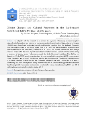We generate mesoscopic patterns by sampling the system with action functional (25) on a two-dimensional domain. The spatial lattice spacing is 0.2 and the normalized (via lattice spacing) microscopic interacting parameters are $k_{A} = k_{B} = 2.25$. The chain length is 100 with $N_{A} = 70$ and $N_{B} = 30$. $n$ is chosen to normalize density $\rho_0 = 1$. Figures 1a, 1b, and 1c show examples of mesoscopic density $\rho_A$ for different interacting parameters $\chi$. Figures 1c and 1d show two different statistical mesoscopic sample patterns for the same interacting parameter $\chi = 0.4$. The density $\rho_B$ is a complementary of $\rho_A$ due to conserved local density. 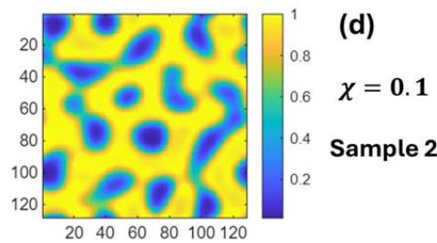    Fig. 1: Mesoscopic Density a for Different Interacting Parameters (a) $\chi = 0.1$, (b) $\chi = 0.4$, (c) $\chi = 1.0$, (d) $\chi = 0.4$. (c) and (d) are two Different Statistical Samples for the same Interacting Parameter $\chi = 0.4$ To evaluate a machine learning algorithm's ability to learn and generate mesoscopic spatial patterns, we begin with training the algorithm with a set of mesoscopic pattern samples. An out-of-sample pattern is then selected, and noise is added to corrupt the original pattern. The trained algorithm is tested on its performance in recovering the original pattern from the noisy version as well as its ability to generate new patterns with similar statistical properties. This assessment uses the scenario above of two interacting species within a domain size of 6.4. 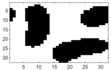In traditional Boltzmann machine learning, connection weights between visible and hidden nodes must be trained on large, statistically similar samples. Figure 2a displays the original mesoscopic pattern generated from two interacting species, while Figure 2b shows a noisy version. Recovering the original pattern requires training with many statistical samples; Figure 2c illustrates a successful recovery using 80 training samples with the same statistics. In contrast, Figure 2d demonstrates that a restricted Boltzmann machine trained with only 10 samples cannot effectively restore the original pattern from noisy data.  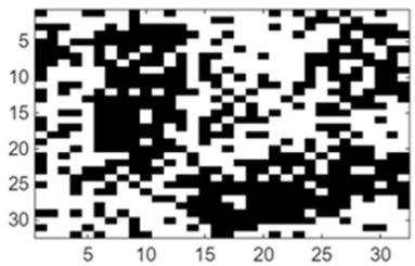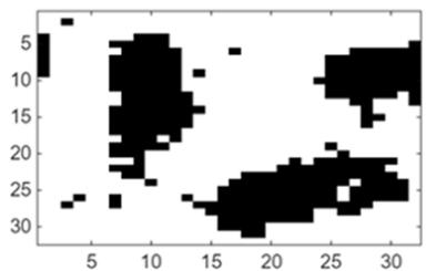(a) (c)   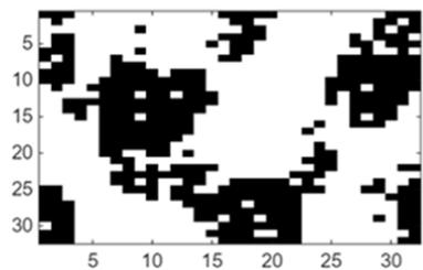 Fig. 2: Restricted Boltzmann machine learning and pattern recovery. (a) Original mesoscopic pattern. (b) Mesoscopic pattern with added noise (c) Recovery of original pattern for a restricted Boltzmann machine trained with 80 samples of the same statistics (d) Recovered pattern for a restricted Boltzmann machine trained with 10 samples of the same statistics For the field solution that integrates machine learning with physics models, we first construct a machine learning neural operator that maps between auxiliary fields (or connection weights) and mesoscopic fields (visible nodes). Figure 3 provides two examples comparing the neural operator predicted mappings with the ground truth. This neural operator is trained solely by the simulated data from the formula $\rho (r) = \frac{1}{Z_m}\frac{\delta Z_m(f)}{\delta f(f)}$ and the microscopic partition function (24), without using any mesoscopic data. 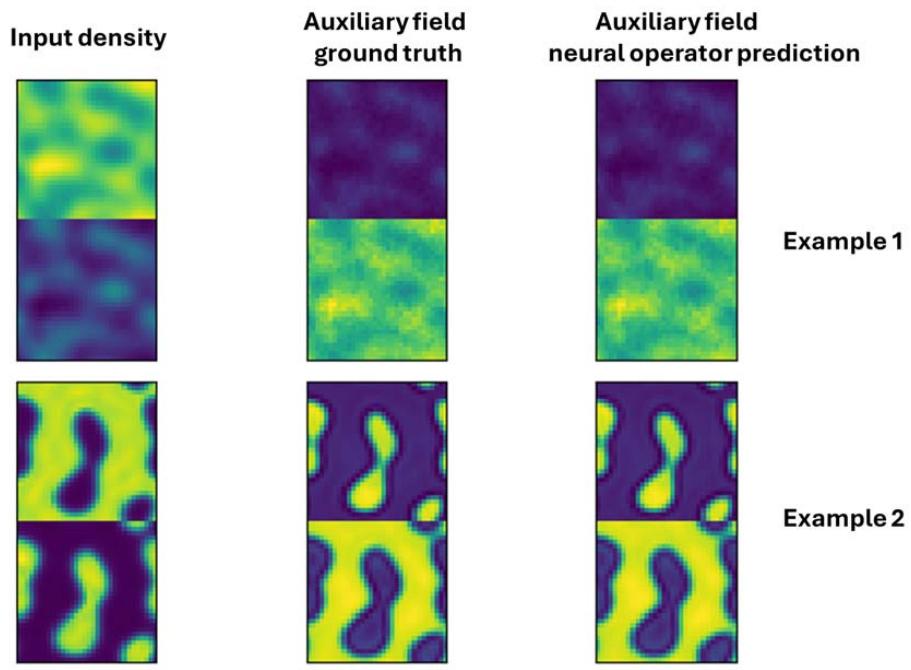 Fig. 3: Neural Operator Functional Mapping between Auxiliary Fields and Mesoscopic Fields With the established neural operator mapping between mesoscopic fields and auxiliary fields, field functional (25) enables the recovery of the original mesoscopic pattern from a noisy input. In the context of machine learning integrated with physical models, typically only one or two original mesoscopic patterns are needed to infer the interaction parameters of actional functional (25). Figure 4 presents an example illustrating the reconstruction of a mesoscopic pattern from a noisy mesoscopic pattern utilizing a field-based approach that combines machine learning with physical models. In addition to recovering the original mesoscopic pattern from observed noisy data, field solutions that integrate machine learning with physical models possess extrapolation capabilities beyond those of conventional machine learning methods. For instance, after recovering the true mesoscopic structure from noisy observations, machine learning with physics model approaches can generate statistical samples of mesoscopic patterns under varying mesoscopic field interaction strengths; without requiring additional data. This capability is unattainable with traditional machine learning frameworks like Boltzmann machines. In the case of restricted Boltzmann machines, generating patterns with different mesoscopic field interactions demands large training data samples for each specific interaction parameter. The restricted Boltzmann machine must relearn weight statistics whenever the underlying mesoscopic pattern distribution changes due to a change of interaction parameter.   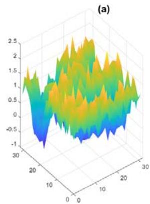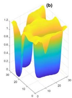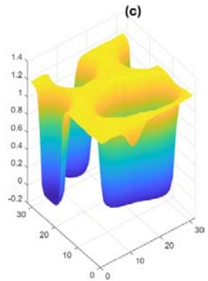 Fig. 4: Learning and pattern recovery of the field solution that integrates machine learning with physics models. (a) Mesoscopic pattern with added noise (b) Original mesoscopic pattern (c) Recovered mesoscopic pattern from field solution that integrates machine learning with physics models; two samples are used to infer the interacting parameter Our field solution, which integrates machine learning with physics models, also enables extrapolation in dynamic evolution. The action functional (22), which is based on system thermodynamics, serves as the free energy of mesoscopic fields $F \sim \beta A$. Once the true mesoscopic structure is recovered from noisy data, our models can analyze how these patterns evolve-for example, by following free energy gradients with local mobility: $$ \frac {\partial \rho}{\partial t} = \nabla \cdot [ M (t, \rho) \nabla \frac {\delta F (\rho , t)}{\delta \rho} ] \tag {26} $$ where $M(t,\rho)$ is a local mobility and $\frac{\delta F(\rho,t)}{\delta\rho}$ is the role of the local free energy gradient. Traditional machine learning methods such as Boltzmann machines cannot perform this type of extrapolation on pattern evolution. Because these models are data-driven, they need to relearn weight statistics using large data samples when mesoscopic pattern distributions change during evolution. ## IV. CONCLUSION We use path integral methods to derive a mesoscopic field solution that unifies machine learning with physics models. In our solution, machine learning architecture and physics models are represented as a unified field entity. Microscopic physics mechanisms are incorporated as machine learning hidden fields and their interactions with the mesoscopic field through auxiliary fields are the connecting weights between machine learning layers. Unlike traditional machine learning models, such as layered Boltzmann machines, instead of imposing statistical assumptions on hidden nodes and learning weight statistics from data, our method derives the hidden fields formalism based on microscopic interaction mechanisms and determines the connecting weights through action functional minimization principle. To enhance machine learning efficiency, we apply the functional neural operator technique to map between auxiliary fields and mesoscopic fields. We demonstrate our solution via a case of mesoscopic patterns generated by two interacting species bonded by a chain structure. By integrating principles from physics models with machine learning methodologies, our approach achieves high performance in learning and generating mesoscopic patterns with limited datasets. This technique effectively captures physical interactions across multiple scales, thereby enabling reliable extrapolation to patterns with varying interaction parameters and dynamic evolution of mesoscopic patterns. The mesoscopic field approach unifying machine learning and physics models can be readily used in diversified areas of physics, material science, biology, and social dynamics. Future research may address complex applications with both limited data and uncertain physical mechanisms, developing efficient algorithms that merge physico-principle based solutions, such as self-consistent action functional minimization and data-driven solutions, such as contrast divergence minimization.

Generating HTML Viewer...