## I. INTRODUCTION Graph theory, a foundational discipline within discrete mathematics, explores graphs comprising vertices (or nodes) connected by edges(or links). These abstract constructs are powerful tools for modeling pair wise relationships across various fields, including computer science, biology, physics, chemistry, transportation, and social network analysis. Graphs enable the representation of systems as diverse as internet connectivity, molecular structures, urban transportation networks, and social interactions. The construction and analysis of specific types of graphs provide deeper insights into the properties and behaviors of these complex systems. This paper presents a computational approach to constructing classic graphs in graph theory using Python programming. The primary objective is to bridge the theoretical framework of graph theory with the practical application of computer programming to foster understanding, visualization, and manipulation of intricate graph structures. With its ease of use, extensive libraries, and built-in graphic capabilities like the turtle module, Python offers a suitable platform for modeling and animating these graphs in an educational and research context. The study focuses on a collection of well-known graphs that hold historical, mathematical, and practical significance. These include the Wagner graph, Desargues graph, Herschel graph, Möbius-Kantor graph, Franklin graph, truncated icosahedral graph, and triangular grid graph. Each graph selected for this project embodies unique structural and topological properties that make it ideal for exploring advanced concepts such as regularity, symmetry, non-planarity, chromatic characteristics, and Hamiltonicity. The Wagner graph, a 3-regular graph with 8 vertices and 12 edges, is a key structure in minor theory used in studying apex and toroidal graphs. Its girth of 4, radius and diameter of 2, and chromatic number of 3 exemplify important constraints in planar graph theory and are instrumental in Ramsey's theory. The Desargues graph, with 20 vertices and 30 edges, is known for its high symmetry and serves as a model in stereochemistry. Its distance-transitive and Hamiltonian nature makes it a powerful object in mathematics and chemistry. This graph also belongs to the family of cubic, distance-regular graphs and exhibits elegant structural harmony. The Herschel graph, though relatively small with 11 vertices and 18 edges, holds significance as the smallest non-Hamiltonian polyhedral graph. It provides a clear example of the limits of Hamiltonian cycles in three-dimensional graph structures and plays a crucial role in understanding planar graph exceptions. The Möbius-Kantor graph, a cubic bipartite symmetric graph with 16 vertices and 24 edges, offers insights into the behavior of generalized Petersen graphs. It is a helpful substructure within higher-dimensional graphs like the hypercube and plays a key role in studying symmetry and Cayley graphs. The Franklin graph, famous for its application to topological coloring problems, was used by Philip Franklin to disprove the Heawood conjecture on the Klein bottle. With 12 vertices and 18 edges, it remains an essential case study in topological graph theory and graph coloring. The truncated icosahedral graph, or the Buckminster Fullerene graph, is derived from an Archimedean solid and features 60 vertices and 90 edges. Its structure models the carbon molecule $C_{60}$ and is widely recognized in chemistry and architecture. As a 3-regular graph, it demonstrates the complexity and symmetry of polyhedral graphs and the feasibility of rendering them computationally. Finally, the triangular grid graph is a visual model for lattice structures. It represents the layout of triangular tilings and has applications in physics, chemistry, and game theory. These graphs are important in modeling networks with hexagonal or triangular symmetry. In this research, each graph is constructed algorithmically using Python's turtle module. The process involves deriving polar coordinates for vertex placement, calculating edge connections using trigonometry, and applying stylized rendering for clear visualization. This computational method enables students and researchers to dynamically visualize and interact with graph properties, fostering deeper engagement with abstract concepts. Additionally, this study incorporates generative artificial intelligence tools, such as ChatGPT, to reproduce and verify Python programs for each graph. Through prompt engineering, the researchers crafted queries that guided the AI in generating accurate code representations of each graph structure. This dual approach-combining manual programming with AI-assisted verification-demonstrates the synergy between human logic and machine learning in computational mathematics. The integration of Python into graph theory education offers numerous pedagogical advantages. It provides a platform for visual experimentation, encourages algorithmic thinking, and bridges the gap between abstract mathematical definitions and concrete visual outputs. Furthermore, using AI tools introduces learners to emerging technologies in computational science, enhancing their digital literacy and programming fluency. This paper aims to serve as both a research contribution and a teaching resource. Illustrating how classic graphs can be constructed through code provides a replicable methodology for instructors and students to explore graph theory in an interactive, project-based environment. Including code, figures, and AI-generated examples supports active learning and promotes inquiry-based exploration. In the following sections, the mathematical characteristics of each selected graph are discussed in detail, followed by their respective Python implementations. Through this work, the authors aim to deepen understanding, inspire further research, and promote computational literacy in graph theory. ## II. METHODOLOGIES This study adopts a computational and algorithmic methodology to construct and analyze classic graphs in graph theory using Python programming. The primary goal is to bridge mathematical abstraction with visual comprehension by implementing graph structures through code. Python's flexibility, particularly its turtle graphics module, is the foundation for this approach, enabling accurate and dynamic graph rendering based on geometric and trigonometric calculations. The methodology follows a systematic, replicable process applied across all selected graphs. Each begins with a thorough mathematical analysis-defining vertex counts, edge arrangements, degrees, symmetries, and other graph invariants. Next, the design transitions to coordinate planning, typically utilizing polar geometry to determine optimal vertex placement around circular or polygonal paths. Edges are drawn between these vertices by calculating precise movements and rotations within the turtle environment. Each Python program is customized to the individual graph's structure. This includes 3-regular graphs like the Wagner and Franklin graphs, symmetric bipartite graphs like the Möbius-Kantor graph, and complex polyhedral graphs like the truncated icosahedral graph. The visualizations often employ color-coded vertices, labeled nodes, and edge stylizations to reflect graph attributes like chromatic number, connectivity, and planarity for enhanced educational value and clarity. In addition to constructing the graphs manually through code, this study integrates generative AI tools, specifically ChatGPT, by using prompt engineering to generate alternative Python implementations. This dual strategy-manual coding followed by AI-assisted reproduction-enabled cross-verification of graphical outputs and exposes learners to collaborative AI programming practices. Overall, this methodology emphasizes reproducibility, educational accessibility, and computational precision. It supports the theoretical exploration of graph properties and enables hands-on learning and experimentation. By merging algorithmic thinking with visual modeling, this framework equips students and researchers with a powerful toolkit for advancing their understanding of graph theory through Python. ## III. 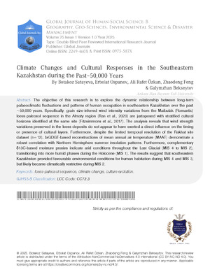WAGNER GRAPH In the mathematical field of graph theory, the Wagner graph is a 3-regular graph with 8 vertices and 12 edges (Bondy & Murty, 2007). It is the 8-vertex Möbius ladder graph. It is nonplanar but has a crossing number of one, making it an apex graph. It can be embedded without crossings on a torus or projective plane and is also a toroidal graph. It has girth 4, diameter 2, radius 2, chromatic number 3, chromatic index 3, and is both 3-vertex-connected and 3-edge-connected. It is a vertex-transitive graph but is not edge-transitive. Its whole automorphism group is isomorphic to the dihedral group $\mathsf{D}_8$ of order 16, the group of an octagon symmetries, including rotations and reflections ("Wagner Graph," 2024). The Wagner graph is triangle-free and has independence number three, providing one half of the proof that the Ramsey number $R(3,4)$ (the least number n such that any n-vertex graph contains either a triangle or a four-vertex independent set) is 9 (Soifer, 2008). Wagner graph has 392 spanning trees; it and the complete bipartite graph $K_{3,3}$ have the most spanning trees among all cubic graphs with the same number of vertices (Jakobson & Rivin, 1999). The Wagner graph is also one of four minimal forbidden minors for the graphs of tree width at most three (the other three being the complete graph $K_{5}$, the graph of the regular octahedron, and the graph of the pentagonal prism) and one of four minimal forbidden minors for the graphs of branch width at most three (the other three being $K_{5}$, the graph of the octahedron, and the cube graph) ("Wagner Graph," 2024; Bodlaender, 1998; Bodlaender & Thilikos, 1999). Wagner's famous conjecture asserts that for any infinite set of graphs, one of its members is isomorphic to a minor of another (all graphs in this paper are finite) (Wagner, 1970). The project proving Wagner's conjecture was started by Robertson and Seymour, later joined by Thomas, and completed in 2004, which led to entirely new concepts and a new way of looking at graph theory (Lovasz, 2006). {"algorithm_caption":[],"algorithm_content":\[{"type":"text","content":"Python Program for Wagner Graph \\nimport turtle \\nimport math \\nt = turtle.Turtle() \\nt.speed("fastest") \\nfor k in range(8): t.penup() x1 = 300\\*math.cos(math.pi\\*((45\\\*k)%360)/180) y1 = 300\\*math.sin(math.pi\\*((45\\\*k)%360)/180) t.goto(x1,y1) t.pendown() x2 = 300\\*math.cos\\{(math.pi\\*((45\\\*k+45)%360)/180) y2 = 300\\*math.sin(math.pi\\*((45\\\*k+45)%360)/180) t.goto(x2,y2) radius = 300 \\nfor k in range(8): t.penup() t.goto(0,0) t.setheading(45\\\*k) t.forward(radius) t.pendown() t fillcolor("blue") t.begin_fill() tcircle(4) t.end_fill() radius = 300 \\nfor k in range(4): t.penup() x1 = radius\\*math.cos(math.pi\\*((45\\\*k)%360)/180) y1 = radius\\*math.sin(math.pi\\*((45\\\*k)%360)/180) t.goto(x1,y1) t.pendown() x2 = radius\\*math.cos\\{(math.pi\\*((45\\\*k+180)%360)/180) y2 = radius\\*math.sin\\} (math.pi\\*((45\\\*k+180)%360)/180) t.goto(x2,y2) t.hideturtle() Using the previous algorithm, we generate the Wagner graph as shown in Figure 1. "}\]} 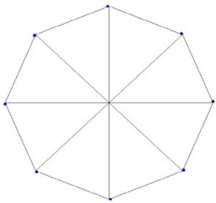 Figure 1: Wagner Graph After uploading the above graph to ChatGPT, we asked, "Based on the attached image/graph, could you develop a Python program to reproduce it?" The Python program generated by ChatGPT produced the following image in Figure 1(a). 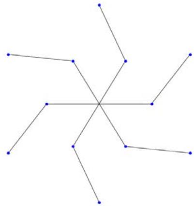 Figure 1(a) After uploading the above graph to ChatGPT, we asked, "Based on the attached image/graph, could you develop a Python program to reproduce it?" The Python program generated by ChatGPT produced the following image in Figure 1(b). 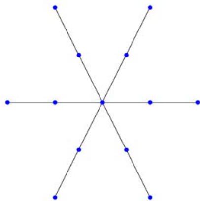 Figure 1(b) ## IV. 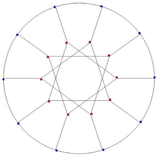DESARGUES GRAPH The Desargues graph is a distance-transitive, cubic graph with 20 vertices and 30 edges. It is named after Girard Desargues, arises from several different combinatorial constructions, has a high level of symmetry, is the only known non-planar cubic partial cube, and has been applied in chemical databases. It is a symmetric graph with symmetries that take any vertex to any other vertex and any edge to any other edge. Its symmetry group has order 240, and is isomorphic to the product of a symmetric group on 5 points with a group of order 2 ("Desargues Graph," 2024). In chemistry, the Desargues graph is known as the Desargues-Levi graph; it is used to organize systems of stereoisomers of 5-ligand compounds. In this application, the thirty edges of the graph correspond to pseudorotations of the ligands ("Desargues Graph," 2024; Balaban, Farcasiu, & Baniača, 1966; Mislow, 1970). It has chromatic number 2, chromatic index 3, radius 5, diameter 5, and girth 6. It is also a 3-vertex-connected and a 3-edge-connected Hamiltonian graph. It has a book thickness of 3 and a queue number of 2 ("Desargues Graph," 2024). All the cubic distance-regular graphs are known (Brouwer, Cohen, & Neumaier, 1989). The Desargues graph is one of the 13 such graphs ("Desargues Graph," 2024). Python Program for Creating Desargues Graph import turtle import math $$ t = turtle.Turtle() $$ $$ t.speed("fastest") $$ $$ t. p e n u p () $$ $$ t. g o t o (0, - 3 0 0) $$ $$ t. p e n d o w (.) $$ $$ t. c i r c l e (3 0 0) $$ $$ \text{radius} = 3 0 0 $$ $$ for k in range(10): $$ $$ t. p e n u p () $$ $$ t. g o t o (0, 0) $$ $$ t. s e t h e a d i n g (3 6 ^ {*} k) $$ $$ t. f o r w a r d (r a d i u s) $$ $$ t. p e n d o w ( $$ $$ t. f i l l c o l e (" b l u e") $$ $$ t. b e g i n \_ f i l l ( $$ $$ t.circle(4) $$ $$ t.end_fill() $$ $$ \text{radius} = 1 5 0 $$ $$ f o r k i n r a n g e (1 0): $$ $$ t. p e n u ( ) $$ $$ t. g o t o (0, 0) $$ t.forward(radius) t.pendown() $$ t.begin_fill(color('red')) $$ $$ t.begin_fill() $$ tcircle(4) $$ t.end_fill() $$ for $k$ in range(10): t PENUP() $$ x 1 = 300 ^ {*} \text {math .} \cos (\text {math .} p i ^ {*} ((36 ^ {*} k) \% 360) / 180) $$ $$ y 1 = 300* \text{math.sin} (\text{math.pi} * ((36* k) \% 360) / 180) $$ $$ t. g o t o (x 1, y 1) $$ $$ t.pendown() $$ $$ x 2 = 150 ^ {*} \text {math . c o s} (\text {math . p i} ^ {*} ((36 ^ {*} k) \% 360) / 180) $$ $$ y 2 = 150* \text{math.sin} (\text{math.pi} * ((36* k) \% 360) / 180) $$ $$ t. g o t o (x 2, y 2) $$ for $k$ in range(10): $$ t.penup() $$ $$ x 1 = 150 ^ {*} \text {math .} \cos (\text {math .} p i ^ {*} ((36 ^ {*} k) \% 360) / 180) $$ $$ y 1 = 150 ^ {*} \text {math. sin} (\text {math. p i} ^ {*} ((36 ^ {*} k) \% 360) / 180) $$ $$ t. g o t o (x 1, y 1) $$ $$ t.pendown() $$ $$ x 2 = 1 5 0 * \text{math . cos} $$ $$ \left(\mathbf{math}. \mathrm{pi} ^ {*} \left(\left(36 ^ {*} \mathrm{k} + 108\right) \% 360\right) / 180\right) $$ $$ y 2 = 1 5 0 * \text{math . sin} $$ $$ \left(\text{math.pi} * \left(\left(36 * k + 108\right) \% 360\right) / 180\right) $$ $$ t. g o t o (x 2, y 2) $$ $$ t. h i d e t u r l e () $$ Using the previous algorithm, we generate the Desargues graph shown in Figure 2.  Figure 2: Desargues Graph After uploading the above graph to ChatGPT, we asked, "Based on the attached image/graph, could you develop a Python program to reproduce it?" The Python program generated by ChatGPT produced the following image in Figure 2 (a). 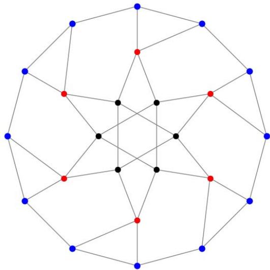 Figure 2 (a) After uploading the above graph to ChatGPT, we asked, "Based on the attached image/graph, could you develop a Python program to reproduce it?" The Python program generated by ChatGPT produced the following image in Figure 2 (b). 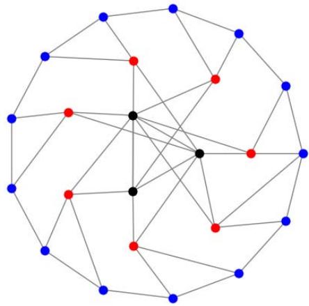 Figure 2 (b) ## V. HERSCHEL GRAPH The Herschel graph is a bipartite undirected graph with 11 vertices and 18 edges. It is a polyhedral graph (the graph of a convex polyhedron). It is the smallest polyhedral graph that does not have a Hamiltonian cycle, a cycle passing through all its vertices. It is named after British astronomer Alexander Stewart Herschel, because Herschel studied Hamiltonian cycles in polyhedral graphs (but not of this graph) (Wikipedia contributors, 2023). Herschel graph has three vertices of degree four and eight vertices of degree three. Each two distinct degree-four vertices share two degree-three neighbors, forming a four-vertex cycle with these shared neighbors. Three of these cycles pass through six of the eight degree-three vertices. Two more degree-three vertices do not participate in these four-vertex cycles; instead, each is adjacent to three of the six vertices (Wikipedia contributors, 2023; Lawson-Perfect, 2013). Herschel's graph also provides an example of a polyhedral graph for which the medial graph has no Hamiltonian decomposition into two edge-disjoint Hamiltonian cycles. The medial graph of the Herschel graph is a 4-regular graph with 18 vertices, one for each edge of the Herschel graph; two vertices are adjacent in the medial graph whenever the corresponding edges of the Herschel graph are consecutive on one of its faces (Wikipedia contributors, 2023; (Bondy & Häggkvist, 1981). {"algorithm_caption":[{"type":"text","content":"Python Program for Creating Herschel Graph "}],"algorithm_content":\[{"type":"text","content":"import turtle t.pendown() \\nimport math t.goto(0,0) \\nt = turtle.Turtle() t.penup() \\nt.speed("fastest") x1 = 300\\*math.cos(math.pi\\*((90\\\*0)%360)/180) \\nt.penup() y1 = 300\\*math.sin(math.pi\\*((90\\\*0)%360)/180) \\nt.goto(0,0) t.goto(x1,y1) \\nt.pendown() t.pendown() \\nt fillscolor("blue") x2 = 150\\*math.cos(math.pi\\*((60\\\*0)%360)/180) \\nt.begin_fill() y2 = 150\\*math.sin(math.pi\\*((60\\\*0)%360)/180) \\nt.circle(4) t.goto(x2,y2) \\nt.end_fill() t.penup() \\nt.penup() x1 = 300\\*math.cos(math.pi\\*((90\\\*1)%360)/180) \\nt.goto(0,-300) y1 = 300\\*math.sin(math.pi\\*((90\\\*1)%360)/180) \\nt.pendown() t.goto(x1,y1) \\nt.circle(300) t.pendown() \\nradius = 300 x2 = 150\\*math.cos(math.pi\\*((60\\\*1)%360)/180) \\nfor k in range(4): y2 = 150\\*math.sin(math.pi\\*((60\\\*1)%360)/180) \\nt.penup() t.goto(x2,y2) \\nt.goto(0,0) t.penup() \\nt.setheading(90\\\*k) x1 = 300\\*math.cos(math.pi\\*((90\\\*1)%360)/180) \\nt.forward(radius) y1 = 300\\*math.sin(math.pi\\*((90\\\*1)%360)/180) \\nt.pendown() t.goto(x1,y1) \\nt fillcolor("blue") t.pendown() \\nt.begin_fill() x2 = 150\\*math.cos(math.pi\\*((60\\\*2)%360)/180) \\ntcircle(4) y2 = 150\\*math.sin(math.pi\\*((60\\\*2)%360)/180) \\nt.end_fill() t.goto(x2,y2) \\nradius = 150 t.penup() \\nfor k in range(6): x1 = 300\\*math.cos(math.pi\\*((90\\\*2)%360)/180) \\nt.penup() y1 = 300\\*math.sin(math.pi\\*((90\\\*2)%360)/180) \\nt.goto(0,0) t.goto(x1,y1) \\nt.setheading(60\\\*k) t.penup() "}\]} t.pendown() t fills color("red") $$ t.begin_fill() $$ tcircle(4) $$ t.end_fill() $$ for $k$ in range(1,3,1): t PENUP() [x1 = 150 * \\text{math.cos(math.pi} \\times (60 * k) % 360/180] y1 = 150*math.sin(math.pi*((60\*k)%360)/180) t.goto(x1,y1) t.pendown() t.goto(0,0) for $k$ in range(4,6,1): t.penup() [x1 = 150 * \\text{math.cos(math.pi} \\times (60 * k) / 360/180] y1 = 150*math.sin(math.pi*((60\*k)%360)/180) t.goto(x1,y1) t.pendown() t.goto(0,0) t.penup() [x1 = 300^{\\star} \\text{math.cos(math.pi}^{\\star}((90^{\\star}0) % 360) / 180)] y1 = 300*math.sin(math.pi*((90\*0)%360)/180) t.goto(x1,y1) t.pendown() [x2 = 150 * \\text{math.cos(math.pi} \\times (60 * 0) % 360/180] y2 = 150*math.sin(math.pi*((60\*0)%360)/180) t.goto(x2,y2) t.penup() [x1 = 300^{\\star} \\text{math.cos(math.pi}^{\\star}((90^{\\star}1)% 360) / 180)] y1 = 300*math.sin(math.pi*((90\*1)%360)/180) t.goto(x1,y1) t.pendown() [x2 = 150^{\\star} \\text{math.cos(math.pi}^{\\star}((60^{\\star}1)%360)/180)] y2 = 150*math.sin(math.pi*((60\*1)%360)/180) t.goto(x2,y2) x1 = 300*math.cos(math.pi*((90\*1)%360)/180) y1 = 300*math.sin(math.pi*((90\*1)%360)/180) [x2 = 150^{\\star} \\text{math.cos(math.pi}^{\\star}((60^{\\star}2)%360)/180)] y2 = 150*math.sin(math.pi*((60\*2)%360)/180) [x1 = 300^{\\star} \\text{math.cos(math.pi}^{\\star}((90^{\\star}2)% 360) / 180)] y1 = 300*math.sin(math.pi*((90\*2)%360)/180) $$ x2 = 150*\text{math.cos} (\text{math.pi}*((60*3)\% 360) / 180) $$ $$ y2 = 150*\mathsf{math.sin}(\mathsf{math.pi}*((60*3)\% 360) / 180) $$ $$ t. g o t o (x 2, y 2) $$ $$ t. p e n u p () $$ $$ x 1 = 300 ^ {*} \text {math . c o s} (\text {math . p i} ^ {*} ((90 ^ {*} 3) \% 360) / 180) $$ $$ y 1 = 300 ^ {*} \text {math.sin} (\text {math.pi} ^ {*} ((90 ^ {*} 3) \% 360) / 180) $$ $$ t. g o t o (x 1, y 1) $$ $$ t.pendown() $$ $$ x2 = 150 ^ {*} \text {math.cos} (\text {math.pi} ^ {*} ((60 ^ {*} 4) \% 360) / 180) $$ $$ y2 = 150*\text{math.sin} (\text{math.pi}*((60*4)\% 360) / 180) $$ $$ t. g o t o (x 2, y 2) $$ $$ t. p e n u p () $$ $$ x 1 = 300 ^ {*} \text {math . c o s} (\text {math . p i} ^ {*} ((90 ^ {*} 3) \% 360) / 180) $$ $$ y 1 = 300 ^ {*} \text {math.sin} (\text {math.pi} ^ {*} ((90 ^ {*} 3) \% 360) / 180) $$ $$ t. g o t o (x 1, y 1) $$ $$ t.pendown() $$ $$ x2 = 150 ^ {*} \text {math.cos} (\text {math.pi} ^ {*} ((60 ^ {*} 5) \% 360) / 180) $$ $$ y2 = 150*\text{math.sin} (\text{math.pi}*((60*5)\% 360) / 180) $$ $$ t. g o t o (x 2, y 2) $$ $$ t. p e n u p () $$ $$ x 1 = 150 ^ {*} \text {math.cos} (\text {math.pi} ^ {*} ((60 ^ {*} 0) \% 360) / 180) $$ $$ y1 = 150*\text{math.sin} (\text{math.pi}*((60*0)\% 360) / 180) $$ $$ t. g o t o (x 1, y 1) $$ $$ t. p e n d o w () $$ $$ x2 = 150 ^ {*} \text {math.cos} (\text {math.pi} ^ {*} ((60 ^ {*} 1) \% 360) / 180) $$ $$ y2 = 150*\text{math.sin} (\text{math.pi}*((60*1)\% 360) / 180) $$ $$ t. g o t o (x 2, y 2) $$ $$ t.penup() $$ $$ x1 = 150 ^ {*} \text {math.cos} (\text {math.pi} ^ {*} ((60 ^ {*} 0) \% 360) / 180) $$ $$ y1 = 150*\text{math.sin} (\text{math.pi}*((60*0)\% 360) / 180) $$ $$ t. g o t o (x 1, y 1) $$ $$ t.pendown() $$ $$ x2 = 150*\text{math.cos} (\text{math.pi}*((60*5)\% 360) / 180) $$ $$ y2 = 150*\text{math.sin} (\text{math.pi}*((60*5)\% 360) / 180) $$ $$ t. g o t o (x 2, y 2) $$ $$ t.penup() $$ $$ x 1 = 150 ^ {*} \text {math . c o s} (\text {math . p i} ^ {*} ((60 ^ {*} 3) \% 360) / 180) $$ $$ y 1 = 150 ^ {*} \text {math.sin} (\text {math.pi} ^ {*} ((60 ^ {*} 3) \% 360) / 180) $$ $$ t. g o t o (x 1, y 1) $$ $$ t. p e n d o w () $$ $$ x2 = 150 ^ {*} \text {math.cos} (\text {math.pi} ^ {*} ((60 ^ {*} 2) \% 360) / 180) $$ $$ y2 = 150^{\star}\mathsf{math.sin}(\mathsf{math.pi}^{\star}((60^{\star}2)\% 360) / 180) $$ $$ t. g o t o (x 2, y 2) $$ $$ t. p e n u p () $$ $$ x 1 = 150 ^ {*} \text {math . c o s} (\text {math . p i} ^ {*} ((60 ^ {*} 3) \% 360) / 180) $$ $$ y 1 = 150 ^ {*} \text {math.sin} (\text {math.pi} ^ {*} ((60 ^ {*} 3) \% 360) / 180) $$ $$ t. g o t o (x 1, y 1) $$ $$ t. p e n d o w () $$ $$ x2 = 150 ^ {*} \text {math.cos} (\text {math.pi} ^ {*} ((60 ^ {*} 4) \% 360) / 180) $$ $$ y2 = 150^{\star}\text{math.sin} (\text{math.pi}^{\star}((60^{\star}4)\% 360) / 180) $$ $$ t. g o t o (x 2, y 2) $$ $$ t. h i d e t u r l e () $$ We generate the Herschel graph shown in Figure 3 using the previous algorithm. 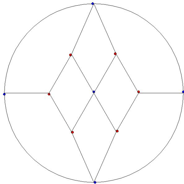 Figure 3: Herschel Graph After uploading the above graph to ChatGPT, we asked, "Based on the attached image/graph, could you develop a Python program to reproduce it?" The Python program generated by ChatGPT produced the following image in Figure 3 (a). 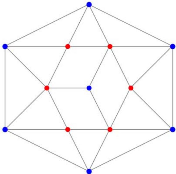 Figure 3 (a) After uploading the above graph to ChatGPT, we asked, "Based on the attached image/graph, could you develop a Python program to reproduce it?" The Python program generated by ChatGPT produced the following image in Figure 3 (b). 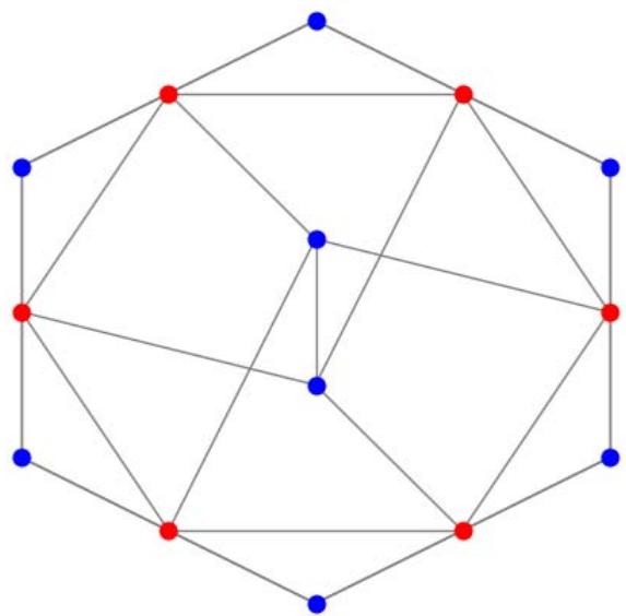 Figure 3 (b) ## VI. MöBIUS-KANTOR GRAPH The Möbius-Kantor graph is a symmetric bipartite cubic graph with 16 vertices and 24 edges named after August Ferdinand Möbius and Seligmann Kantor. It can be defined as the generalized Petersen graph $G(8,3)$: that is, it is formed by the vertices of an octagon, connected to the vertices of an eight-point star in which each point of the star is connected to the points three steps away from it (Wikipedia contributors, 2024). Möbius-Kantor graph is a subgraph of the four-dimensional hypercube graph, formed by removing eight edges from the hypercube. Since the hypercube is a unit distance graph, the Möbius-Kantor graph can also be drawn in the plane with all edges unit length, although such a drawing will necessarily have some pairs of crossing edges. The Möbius-Kantor graph also often occurs as an induced subgraph of the Hoffman-Singleton graph. Each of these instances is, in fact, an eigenvector of the Hoffman-Singleton graph, with an associated eigenvalue of -3. Each vertex not in the induced Möbius-Kantor graph is adjacent to exactly four vertices in the Möbius-Kantor graph, two each in half of a bipartition of the Möbius-Kantor graph. The Möbius-Kantor graph cannot be embedded without crossings in the plane; it has crossing number 4, and is the smallest cubic graph with that crossing number (Wikipedia contributors, 2024; Coxeter, 1950). The automorphism group of the Möbius-Kantor graph is a group of order 96. It acts transitively on the graph's vertices, edges, and arcs. Therefore, the Möbius-Kantor graph is a symmetric graph. It has automorphisms that take any vertex to any other vertex and any edge to any other edge. According to the Foster census, the Möbius-Kantor graph is the unique cubic symmetric graph with 16 vertices, and the smallest cubic symmetric graph is not also distance- transitive. The Möbius-Kantor graph is also a Cayley graph (Wikipedia contributors, 2024). Python Program for Creating Möbius-Kantor Graph import turtle import math $\mathbf{t} =$ turtle.Turtle() t.speed("fastest") t PENUP() t.goto(0,-300) t.pendown() tcircle(300) radius $= 300$ for $k$ in range(8): t.penup() t.goto(0,0) $$ t.setheading(45\*k) $$ t.forward(radius) turtle.pendown() t.fillcolor("blue") $$ t.begin_fill() $$ t.circle(4) $$ t.end_fill() $$ radius $= 150$ for $k$ in range(8): t.penup() # Move pen up t.goto(0,0) $$ t.setheading(45\*k) $$ t.forward(radius) t.fillcolor("red") t.fillcolor("red") $$ t.begin_fill() $$ t.circle(4) $$ t.end_fill() $$ for $k$ in range(8): t.penup() x1 = 150*math.cos(math.pi*((45\*k)%360)/180) y1 = 150*math.sin(math.pi*((45\*k)%360)/180) $\\mathrm{x2} = 300^{\\star}$ math.cos\\ $$ math.pi\*((45\*k+45)%360)/180) $$ y2 = 300*math.sin(math.pi*((45\*k+45)%360)/180) $$ math.pi\*((45\*k+45)%360)/180) $$ for $k$ in range(4): [x1 = 150 * \\text{math.cos(math.pi} \\times ((45 * k) % 360) / 180)] y1 = 150*math.sin(math.pi*((45\*k)%360)/180) {"algorithm_caption":[],"algorithm_content":\[{"type":"text","content":"t.pendown() "},{"type":"equation_inline","content":"x2 = 150^{*}"},{"type":"text","content":" math.cos \\n(math.pi\\*\\*((45\\*k+135)%360)/180) "},{"type":"equation_inline","content":"\\mathbf{y}2 = 150^{\\star}"},{"type":"text","content":" math.sin \\n(math.pi\\*\\*((45\\*k+135)%360)/180) t.goto(x2,y2) \\nfor k in range(4): t PENUP() x1 "},{"type":"equation_inline","content":"= 150^{*}"},{"type":"text","content":" math.cos(math.pi\\*(((45\\*k)%360)/180) y1 "},{"type":"equation_inline","content":"= 150^{*}"},{"type":"text","content":" math.sin(math.pi\\*(((45\\*k)%360)/180) t.goto(x1,y1) t.pendown() x2 "},{"type":"equation_inline","content":"= 150^{*}"},{"type":"text","content":" math.cos \\n(math.pi\\*(((45\\*k+225)%360)/180) y2 "},{"type":"equation_inline","content":"= 150^{\\star}"},{"type":"text","content":" math.sin \\n(math.pi\\*(((45\\*k+225)%360)/180) t.goto(x2,y2) \\nt.penup() x1 "},{"type":"equation_inline","content":"= 150^{*}"},{"type":"text","content":" math.cos(math.pi\\*(((45\\*4)%360)/180) y1 "},{"type":"equation_inline","content":"= 150^{\\star}"},{"type":"text","content":" math.sin(math.pi\\*(((45\\*4)%360)/180) t.goto(x1,y1) \\nt.pendown() x2 "},{"type":"equation_inline","content":"= 150^{*}"},{"type":"text","content":" math.cos(math.pi\\\*(((45\\*7)%360)/180) y2 "},{"type":"equation_inline","content":"= 150^{\\star}"},{"type":"text","content":" math.sin(math.pi\\*(((45\\\*7)%360)/180) t.goto(x2,y2) \\nt.hideturtle()"}\]} Using the previous algorithm, we generate Möbius the Möbius-Kantor graph as shown in Figure 4. 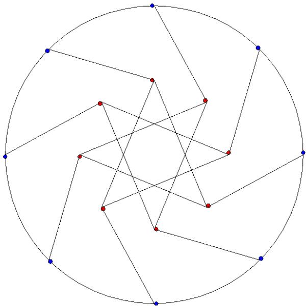 Figure 4: Möbius-Kantor graph After uploading the above graph to ChatGPT, we asked, "Based on the attached image/graph, could you develop a Python program to reproduce it?" The Python program generated by ChatGPT produced the following image in Figure 4 (a). 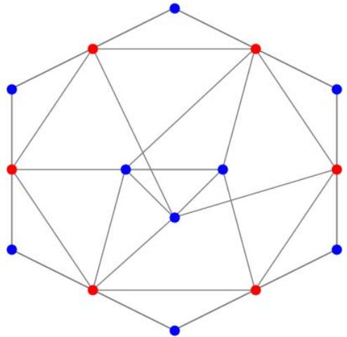 Figure 4 (a) After uploading the above graph to ChatGPT, we asked, "Based on the attached image/graph, could you develop a Python program to reproduce it?" The Python program generated by ChatGPT produced the following image in Figure 4 (b). 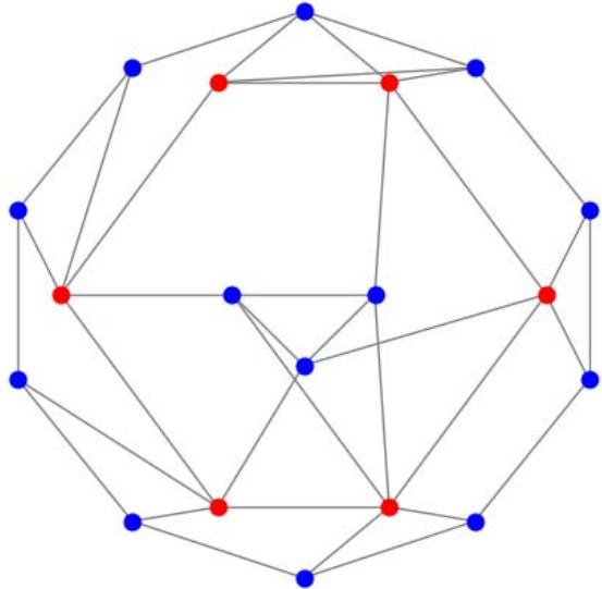 Figure 4 (b) ## VII. FRANKLIN GRAPH The Franklin graph is a 3-regular graph with 12 vertices and 18 edges. Franklin graph is named after Philip Franklin, who disproved the Heawood conjecture on the number of colors needed when a two-dimensional surface is partitioned into cells by a graph embedding (Wikipedia contributors, 2022; Franklin, 1934). The Heawood conjecture implied that the maximum chromatic number of a map on the Klein bottle should be seven, but Franklin proved that in this case six colors always suffice. (The Klein bottle is the only surface for which the Heawood conjecture fails.) The Franklin graph can be embedded in the Klein bottle so that it forms a map requiring six colors, showing that six colors are sometimes necessary in this case. Franklin graph is Hamiltonian and has chromatic number 2, chromatic index 3, radius 3, diameter 3 and girth 4. It is also a 3-vertex-connected and 3-edge-connected perfect graph (Wikipedia contributors, 2022). {"algorithm_caption":[{"type":"text","content":"Python Program for Creating Franklin Graph "}],"algorithm_content":\[{"type":"text","content":"import turtle \\nimport math \\nt = turtle.Turtle() \\nt.speed("fastest") \\nt.pensize(1) \\nfor k in range(12): t.penup() x1 = 300\\*math.cos(math.pi\\*(30\\\*k)%360)/180) y1 = 300\\*math.sin(math.pi\\*(30\\\*k)%360)/180) t.goto(x1,y1) t.pendown() x2 = 300\\*math.cos\\ \\n(math.pi\\*(30\\\*k+30)%360)/180) y2 = 300\\*math.sin\\ \\n(math.pi\\*(30\\\*k+30)%360)/180) t.goto(x2,y2) \\nradius = 300 \\nfor k in range(12): t.penup() t.goto(0,0) t.setheading(30\\\*k) t.forward(radius) t.pendown() t fillcolor("blue") t.begin_fill() tcircle(4) t.end_fill() \\nradius = 300 \\nfor k in range(0,12,2): t.penup() x1 = radius\\*math.cos(math.pi\\*(30\\\*k)%360)/180) y1 = radius\\*math.sin(math.pi\\*(30\\\*k)%360)/180) t.goto(x1,y1) t.pendown() x2 = radius\\*math.cos\\ \\n(math.pi\\*(30\\\*k+150)%360)/180) y2 = radius\\*math.sin\\ \\n(math.pi\\*(30\\\*k+150)%360)/180) t.goto(x2,y2) \\nt.hideturtle() "}\]} Using the previous algorithm we generate the Franklin graph as shown in Figure 5. 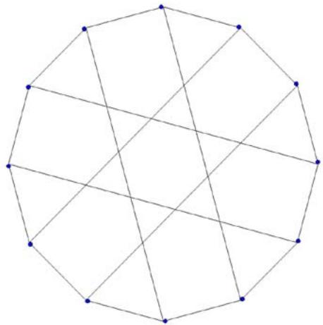 Figure 5: Franklin graph After uploading the above graph to ChatGPT, we asked, "Based on the attached image/graph, could you develop a Python program to reproduce it?" The Python program generated by ChatGPT produced the following image in Figure 5 (a). 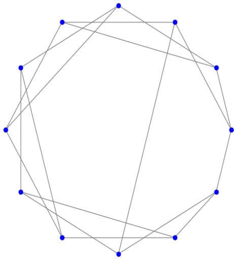 Figure 5 (a) After uploading the above graph to ChatGPT, we asked, "Based on the attached image/graph, could you develop a Python program to reproduce it?" 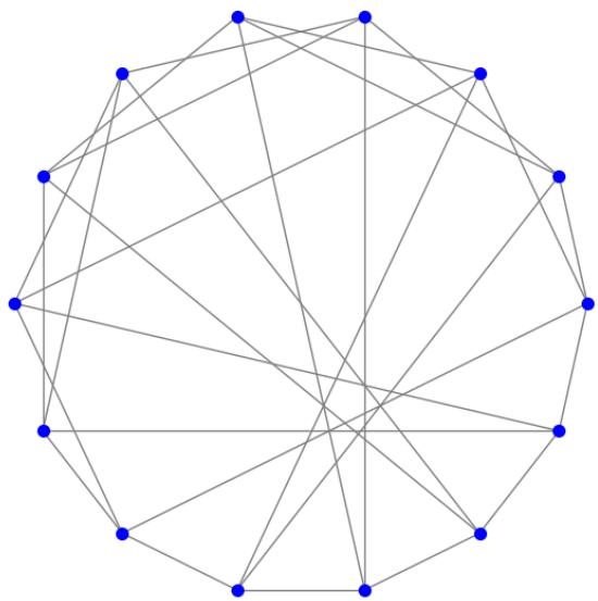 Figure 5 (b) ## VIII. TRUNCATED ICOSAHEDRAL GRAPH In geometry, the truncated icosahedron is a polyhedron that can be constructed by truncating all of the regular icosahedron's vertices. Intuitively, it may be regarded as footballs (or soccer balls) that are typically patterned with white hexagons and black pentagons. It can be found in the application of geodesic dome structures such as those whose architecture Buckminster Fuller pioneered are often based on this structure. It is an example of an Archimedean solid, as well as a Goldberg polyhedron (Weisstein, 2025). According to Steinitz's theorem, the skeleton of a truncated icosahedron, like that of any convex polyhedron, can be represented as a polyhedral graph, meaning a planar graph (one that can be drawn without crossing edges) and 3-vertex-connected graph (remaining connected whenever two of its vertices are removed). The graph is known as truncated icosahedral graph, with 60 vertices and 90 edges. It is an Archimedean graph because it resembles one of the Archimedean solids. It is a cubic graph, meaning that each vertex is incident to exactly three edges. It is sometimes known as the Buckminster Fullerene graph (Weisstein, 2025; Wikipedia contributors, 2024). Python Program for Creating truncated icosahedral graph import turtle 20-gons for $k$ in range(20): t.setheading(18\*k) t.forward(300) t.fillcolor("black") $$ t.begin_fill() $$ circle(4) $$ t.end_fill() $$ t.penup() [x1 = 300^{\\star} \\text{math.cos(math.pi}^{\\star}((18^{\\star}k)% 360) / 180)] y1 = 300*math.sin(math.pi*((18\*k)%360)/180) t.goto(x1,y1) t.setposition(x1,y1) t.pendown() letter = str(k+1) t.color('black') t.write(letter, align='right', font=('Verdana', 13)) "normal") t.color('black') x2 = 300 * math.cos(math.pi * ((18 * k + 18)% 360) / 180) (math.pi\*( $(18^{*}k + 18)\% 360) / 180$ y2 = 300*math.sin(math.pi*((18\*k+18)%360)/180) t.goto(x2,y2) 20 red vertices for $k$ in range(20): t.penup() t.goto(0,0) t.setheading(18\*k) t.forward(240) t.pendown() t.fillcolor('red') $$ t.begin_fill() $$ tcircle(4) $$ t.end_fill() $$ [x1 = 240^{\\star} \\text{math.cos(math.pi}^{\\star}((18^{\\star}k)%360)/180)] y1 = 240 * math.sin(math.pi * ((18 * k)% 360) / 180) t.goto(x1,y1) t.setposition(x1,y1) t.pendown() letter $= \operatorname{str}\left( {{20} + k + 1}\right)$ t.color('red') t.write(letter, align="right", font=("Verdana", 13, "normal") t.color('black') radius $= 180$ for $k$ in range(10): {"code_caption":[],"code_content":\[{"type":"text","content":"t fills color("blue") \\nt.begin_fill() \\ntcircle(4) \\nt.end_fill() \\nx1 = 180*math.cos(math.pi*((36*k)%360)/180) \\ny1 = 180*math.sin(math.pi\*((36*k)%360)/180) \\nt.goto(x1,y1) \\nt.setposition(x1,y1) \\nt.pendown() \\nletter = str(40+k+1) \\nt.color('blue') \\nt.write(letter, align="right", font=("Verdana", 13, "normal")) \\nt.color('black') \\n# 10 green vertices \\nradius = 120 \\nfor k in range(10): \\n t PENUP() \\n t.goto(0,0) \\n t.setheading(36*k) \\n t.forward(radius) \\n t.pendown() \\n t fillcolor("green") \\n t.begin_fill() \\n t.circle(4) \\n t.end_fill() \\n x1 = 120*math.cos(math.pi*((36*k)%360)/180) \\n y1 = 120*math.sin(math.pi\*((36*k)%360)/180) \\n t.goto(x1,y1) \\n t.setposition(x1,y1) \\n t.pendown() \\n letter = str(50+k+1) \\n t.color('green') \\n t.write(letter, align="right", font=("Verdana", 13, "normal")) \\n t.color('black') \\n#edges between black and red vertices \\nfor k in range(0,19,2): \\n t.penup() \\n x1 = 300*math.cos(math.pi\*((18*k)%360)/180) \\n y1 = 300*math.sin(math.pi\*((18*k)%360)/180) \\n t.goto(x1,y1) \\n t.pendown() \\n t.color('red') \\n x2 = 240*math.cos(math.pi\*((18*k+18)%360)/180) \\n y2 = 240*math.sin(math.pi\*((18*k+18)%360)/180) \\n t.goto(x2,y2) \\n t.color('black') \\nfor k in range(0,19,2): "}\],"code_language":"txt"} {"code_caption":[],"code_content":\[{"type":"text","content":"t.penup() x1 = 240*math.cos(math.pi\*((18*k)%360)/180) y1 = 240*math.sin(math.pi\*((18*k)%360)/180) t.goto(x1,y1) t.pendown() t.color('green') x2 = 300*math.cos\\ \\n(math.pi\*((18*k+18)%360)/180) y2 = 300*math.sin(math.pi\*((18*k+18)%360)/180) t.goto(x2,y2) t.color('black') \\n# edges between red vertices \\nfor k in range(1,20,2): t.penup() x1 = 240*math.cos(math.pi\*((18*k)%360)/180) y1 = 240*math.sin(math.pi\*((18*k)%360)/180) t.goto(x1,y1) t.pendown() x2 = 240*math.cos\\ \\n(math.pi\*((18*k+18)%360)/180) y2 = 240*math.sin(math.pi\*((18*k+18)%360)/180) t.goto(x2,y2) \\n#edges between red and blue vertices \\nfor k in range(10): t.penup() x1 = 180*math.cos(math.pi\*((36*k)%360)/180) y1 = 180*math.sin(math.pi\*((36*k)%360)/180) t.goto(x1,y1) t.pendown() x2 = 240*math.cos(math.pi\*((2*18*k)%360)/180) y2 = 240*math.sin(math.pi*((2*18*k)%360)/180) t.goto(x2,y2) \\nfor k in range(10): t.penup() x1 = 180*math.cos(math.pi*((36*k)%360)/180) y1 = 180*math.sin(math.pi\*((36*k)%360)/180) t.goto(x1,y1) t.pendown() x2 = 240*math.cos\\ \\n(math.pi\*((2*18*k+54)%360)/180) y2 = 240*math.sin(math.pi*((2*18*k+54)%360)/180) t.goto(x2,y2) \\n# edges between blue and green vertices \\nfor k in range(10): t.penup() x1 = 180*math.cos(math.pi*((36*k)%360)/180) y1 = 180*math.sin(math.pi\*((36\*k)%360)/180) t.goto(x1,y1) t.pendown() "}\],"code_language":"txt"} $$ x 2 = 120 ^ {*} \text {math . c o s} (\text {math . p i} ^ {*} ((36 ^ {*} k) \% 360) / 180) $$ $$ y2 = 120^{\star}\text{math.sin} (\text{math.pi}^{*}((36^{\star}\mathrm{k})\% 360) / 180) $$ $$ t. g o t o (x 2, y 2) $$ # edges between green and green vertices for $k$ in range(0,10,2): t PENUP() $$ x 1 = 120 ^ {*} \text {math . c o s} (\text {math . p i} ^ {*} ((36 ^ {*} k) \% 360) / 180) $$ $$ y 1 = 120 ^ {*} \text {math.sin} (\text {math.pi} ^ {*} ((36 ^ {*} k) \% 360) / 180) $$ t.goto(x1,y1) t.pendown() $$ x 2 = 1 2 0 ^ {*} \text {m a t h . c o s} $$ $$ (\mathsf{math.pi}^{\star}((36^{*}\mathsf{k} + 72)\% 360) / 180) $$ $$ y2 = 120^{\star}\text{math.sin} (\text{math.pi}^{\star}((36^{\star}\mathrm{k} + 72)\% 360) / 180) $$ t.goto(x2,y2) for $k$ in range(1,10,2): t PENUP() $$ x 1 = 120 ^ {*} \text {math . c o s} (\text {math . p i} ^ {*} ((36 ^ {*} k) \% 360) / 180) $$ $$ y 1 = 120 ^ {*} \text {math.sin} (\text {math.pi} ^ {*} ((36 ^ {*} k) \% 360) / 180) $$ t.goto(x1,y1) t.pendown() $$ x 2 = 1 2 0 ^ {\star} \text {m a t h . c o s} $$ $$ \left(\mathbf{math}. \mathbf{pi} ^ {*} \left(\left(36 ^ {*} k + 72\right) \% 360\right) / 180\right) $$ $$ y2 = 120^{\star}\text{math.sin} (\text{math.pi}^{\star}((36^{\star}\mathrm{k} + 72)\% 360) / 180) $$ t.goto(x2,y2) t.hideturtle() Using the previous algorithm we generate the truncated icosahedral graph as shown in Figure 6. 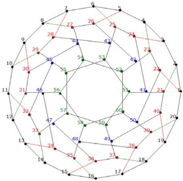 Figure 6: Truncated icosahedral graph After uploading the above graph to ChatGPT, we asked, "Based on the attached image/graph, could you develop a Python program to reproduce it?" The Python program generated by ChatGPT produced the following image in Figure 6 (a). 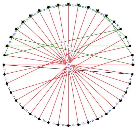 Figure 6 (a) After uploading the above graph to ChatGPT, we asked, "Based on the attached image/graph, could you develop a Python program to reproduce it?" The Python program generated by ChatGPT produced the following image in Figure 5 (b). 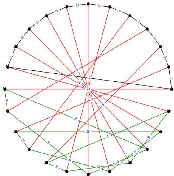 Figure 6 (b) ## IX. TRIANGULAR GRID GRAPH The triangular grid graph $T_{n}$ is the lattice graph obtained by interpreting the order- $(n + 1)$ triangular grid as a graph, with the intersection of grid lines being the vertices and the line segments between vertices being the edges. Equivalently, it is the graph on vertices $(i,j,k)$ with $i,j,k$ being nonnegative integers summing to $n$ such that vertices are adjacent if the sum of absolute differences of the coordinates of two vertices is 2. The graph bandwidth of $T_{n}$ is $n + 1$. $T_{n}$ is also the hexagonal king graph of order $n$, i.e., the connectivity graph of possible moves of a king chess piece on a hexagonal chessboard (West, 2000; Weisstein, 2025). {"algorithm_caption":[],"algorithm_content":\[{"type":"text","content":"Python Program for Creating "},{"type":"equation_inline","content":"T\_{n}"},{"type":"text","content":" \\nimport turtle \\nimport math \\nt = turtle.Turtle() \\nt.speed("fastest") \\ndef Triangular_Grid_Grid(n): size "},{"type":"equation_inline","content":"= 600 / /\\mathfrak{n}"},{"type":"text","content":" \\nfor k in range(0, n+1): x_cor "},{"type":"equation_inline","content":"= -300 + k^{*}"},{"type":"text","content":" size for i in range "},{"type":"equation_inline","content":"(\\mathrm{k} + 1)"},{"type":"text","content":".. t.penup() t.goto(x_cor,300-i*size\\*math.sqrt(3)/2) t.pendown() t fillcolor("red") t.begin_fill () t.cire(2) t.end_fill () x_cor "},{"type":"equation_inline","content":"="},{"type":"text","content":" x_cor - size/2 \\nt.color('black') \\nfor k in range(0, n): x_cor "},{"type":"equation_inline","content":"= -300 + k^{*}"},{"type":"text","content":" size for i in range "},{"type":"equation_inline","content":"(\\mathrm{k} + 1)"},{"type":"text","content":".. t.penup() t.goto(x_cor,300-i*size\\*math.sqrt(3)/2) t.setposition(x_cor,300-i*size\\*math.sqrt(3)/2) t.pendown() t.goto(x_cor + size,300-i*size\\*math.sqrt(3)/2) x_cor "},{"type":"equation_inline","content":"="},{"type":"text","content":" x_cor - size/2 \\nfor k in range(0, n): x_cor "},{"type":"equation_inline","content":"= -300 + k^{*}"},{"type":"text","content":" size for i in range "},{"type":"equation_inline","content":"(\\mathrm{k} + 1)"},{"type":"text","content":".. t.penup() t.goto(x_cor,300-i*size\\*math.sqrt(3)/2) t.setposition(x_cor,300-i*size\\\*math.sqrt(3)/2) t.pendown() t.goto(x_corr + size/2,300(i+1)*size\\*math.sqrt(3)/2) x_cor "},{"type":"equation_inline","content":"="},{"type":"text","content":" x_cor - size/2 \\nfor k in range(0, n): x_cor "},{"type":"equation_inline","content":"= -300 + (k + 1)^{*}"},{"type":"text","content":" size for i in range "},{"type":"equation_inline","content":"(\\mathrm{k} + 1)"},{"type":"text","content":".. t.penup() t.goto(x_cor,300-i*size\\*math.sqrt(3)/2) t.setposition(x_cor,300-i*size\\\*math.sqrt(3)/2) t.pendown() t.goto(x_corr-size/2,300(i+1)\*size\\\*math.sqrt(3)/2) x_cor "},{"type":"equation_inline","content":"="},{"type":"text","content":" x_cor - size/2 \\nt.hideturtle() "}\]} Using the previous algorithm we generate the truncated icosahedral graphs $T_{15}$ and $T_{30}$ as shown in Figure 7-A and Figure 7-B, respectively. 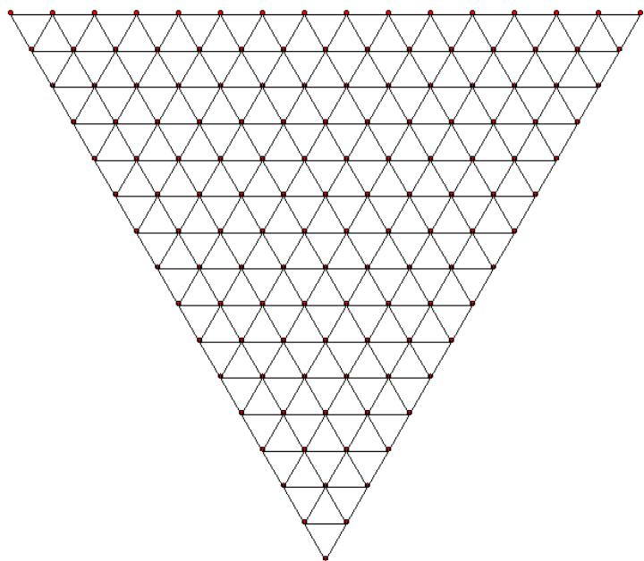 Figure 7-A: Truncated Icosahedral Graph $T_{15}$ 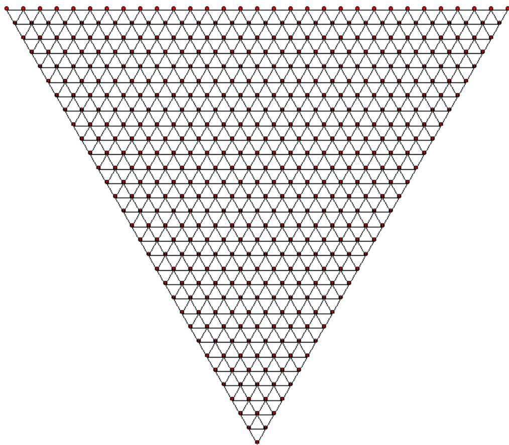 Figure 7-B: Truncated Icosahedral Graph $T_{30}$ After uploading the above graph to ChatGPT, we asked, "Based on the attached image/graph, could you develop a Python program to reproduce it?" The Python program generated by ChatGPT produced the following image in Figure 7-B (a). 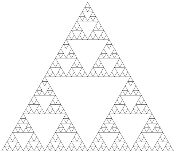 Figure 7-B (a) After uploading the above graph to ChatGPT, we asked, "Based on the attached image/graph, could you develop a Python program to reproduce it?" The Python program generated by ChatGPT produced the following image in Figure 7-B (b).  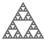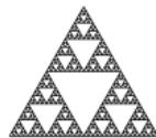  Figure 7-B (b) ## X. INTEGRATING KNOWLEDGE MANAGEMENT INTO COMPUTATIONAL GRAPH THEORY EDUCATION Knowledge management (KM) is pivotal in bridging theory and application in computational graph theory, particularly when using Python to model complex mathematical structures. As graph construction increasingly leverages algorithmic logic and programming, effective KM strategies are essential for facilitating interdisciplinary learning, enhancing educational outcomes, and optimizing research processes. The Knowledge Management Mesosystem Model (Gao & Gao, in press) offers a structured framework that supports the integration of human expertise, algorithmic design, and AI-assisted discovery in educational environments. It comprises three interdependent layers: the Knowledge/Human Layer, the Yin-Yang Knowledge Development and Sharing Layer, and the Data/Machine Layer. These layers align well with the iterative process of coding, testing, and visualizing graphs, allowing students and researchers to transition seamlessly between theory development and practical application. Instructors can cultivate higher-order thinking, collaboration, and computational creativity by incorporating KM strategies into graph theory education. Gao et al. (2025) emphasize the role of innovative teaching practices in business analytics, which mirror similar approaches in computational mathematics where hands-on programming tasks and active learning deepen student engagement. Moreover, integrating AI into KM workflows allows for more dynamic interaction between human logic and machine-generated insights, facilitating advanced problem-solving and deeper conceptual understanding (Gao et al., 2024). Russ (2021) further highlights the necessity of sustainable KM in technology-driven disciplines, underscoring how ethical AI usage and data governance must accompany algorithmic exploration. The symbiotic relationship between knowledge creation and dissemination within KM frameworks is crucial when teaching programming-based graph construction, where students learn from existing models and contribute to evolving digital knowledge ecosystems. In summary, embedding KM principles into computational graph theory enriches the learning experience, encourages innovation, and ensures a sustainable, interdisciplinary approach to knowledge generation in the era of intelligent technologies. ## XI. RESPONSIBLE INTEGRATION OF AI IN COMPUTATIONAL RESEARCH AND EDUCATION As artificial intelligence (AI) becomes more integrated into educational and research contexts, adopting a balanced and responsible approach to its use is essential. In computational fields such as graph theory, AI can support algorithm development, automate visualization, and even suggest code for complex graph structures. However, using AI wisely means recognizing its role as a complement to not a replacement for human logic, creativity, and critical thinking. Gao et al. (2024) highlights that while AI can generate solutions and assist in mathematical reasoning, it must be tempered with human oversight to ensure accuracy, especially in domains requiring rigorous proofs and logical consistency. Misusing generative AI—such as uncritically accepting outputs without validation—can lead to erroneous conclusions and undermine academic integrity. The Knowledge Management Mesosystem Model (Gao & Gao, in press) provides a helpful framework for guiding wise AI integration. Its Data/Machine Layer emphasizes AI-assisted learning while maintaining a strong role for human decision-making. Ethical considerations, data governance, and contextual understanding must be part of any AI-driven educational or research activity. Furthermore, wise AI use aligns with Russ's (2021) model of sustainable knowledge management, which calls for thoughtful integration of technology to enhance-not replace-human cognitive processes. In a programming-rich environment like Python-based graph construction, students and researchers should use AI to augment their understanding: generating baseline code, debugging, or exploring design variations while still being actively involved in problem-solving and model evaluation. Ultimately, using AI wisely means fostering an interdisciplinary mindset where machine intelligence supports but does not eclipse human reasoning. When guided by ethical principles and pedagogical goals, AI can significantly enhance the teaching, learning, and research of mathematical and computational topics. ## XII. PROMPT ENGINEERING AND ITS ROLE IN GRAPH CONSTRUCTION Prompt engineering, the art of crafting precise and effective instructions to guide large language models (LLMs), has become essential in leveraging generative artificial intelligence for diverse tasks, including mathematical problem-solving and programming support. In the context of this study, prompt engineering was pivotal in engaging tools like ChatGPT to recreate Python visualizations of classic graphs in graph theory. By formulating well-structured prompts-such as asking for a Python program to replicate a given graph image-researchers could derive functional code outputs that accurately reproduced complex structures like the Wagner and Desargues graphs. The power of prompt engineering lies in its ability to direct AI toward high-quality, context-aware responses. As Hernández et al. (2024) described, successful interactions with LLMs depend heavily on clarity, specificity, and contextual cues within the prompt. Their work provides over 100 examples, demonstrating that prompt quality significantly impacts response effectiveness across domains. Similarly, Mastering Generative AI and Prompt Engineering underscores that prompt engineering enhances productivity and creativity by allowing users to customize AI output to specific goals, such as generating reproducible code or verifying mathematical properties (Data Science Horizons, 2024). In graph theory education and computational research, prompt engineering bridges human intent and machine-generated assistance. It transforms LLMs from passive responders into collaborative problem-solvers capable of producing code that is not only syntactically correct but also aligned with theoretical graph attributes. As Python continues to serve as a primary medium for algorithmic exploration, prompt engineering empowers both students and researchers to interact more effectively with AI models, thus streamlining the process of constructing, analyzing, and visualizing graphs. ## XIII. CONCLUSION In the Information Age where information inflows and outflows are rapid, complex, and dynamically interspersed within highly uncertain environments, the imperative nature of the necessity for algorithmic learning in higher education has become increasingly clear. Not only is algorithmic learning considered to be integral within the Information and Communications Technology (ICT) domain (Byrka, Sushchenko, Luchko, Perun, & Luchko, 2024), but it is among the most sought after skill for millennials (Ananiadou & Claro, 2009). More importantly, the inculcation of algorithmic learning can help reify an otherwise esoteric way of thinking and, therefore, learning, by helping students organize their thoughts logically in a stepwise fashion. This research has demonstrated how classic graphs in graph theory can be effectively constructed, visualized, and analyzed using Python programming. By focusing on historically significant and mathematically rich graphs such as the Wagner, Desargues, Herschel, Möbius-Kantor, Franklin, truncated icosahedral, and triangular grid graphs, this study bridges the gap between abstract mathematical theory and tangible computational implementation. Python's turtle module proved to be a valuable tool for graph rendering, offering a visually intuitive means of exploring structural properties such as regularity, symmetry, Hamiltonicity, and chromatic characteristics. Using trigonometric and geometric reasoning in these Python scripts encourages learners to connect theoretical graph definitions with algorithmic design, deepening mathematical understanding and programming skills. A significant contribution of this study is the integration of generative AI, particularly ChatGPT, through prompt engineering to reproduce and verify Python code for graph construction. This dual approach validates the manually written code and introduces learners to collaborative human-AI workflows in computational mathematics. Prompt engineering emerged as a vital skill in effectively guiding AI tools, enabling the generation of meaningful and accurate programming solutions aligned with graph-theoretic goals. Moreover, this paper underscores the educational potential of combining coding with visual mathematics. Students and researchers gain a deeper appreciation for graph properties and computational logic by implementing classic graphs in Python. The methodology presented here is replicable and scalable, making it ideal for classroom use, student research, and interdisciplinary applications across science, engineering, and computer science. Ultimately, this work contributes a practical and pedagogically sound approach to teaching and exploring graph theory. Hands-on programming and responsible AI integration fosters computational literacy and inspires further innovation at the intersection of mathematics, computer science, and education. ### Data Availability Conflicts of Interest The authors declare no conflicts of interest. #### Funding Statement This study did not receive any funding in any form. #### ACKNOWLEDGMENT This paper was inspired and initiated by the talks, posters, and conversations at PyCon US 2024, held in Pittsburgh, Pennsylvania, from May 17 to 19, 2024. The first author attended the conference with financial support from the organizers. The work also drew upon his teaching materials for Introduction to Computing at the University of Richmond and Computer Programming I & II at Virginia State University. Part of the research was conducted during his visit to Elizabeth City State University (ECSU) from July 14 to 19, 2024, supported by an ECSU mini-grant. Additional insights were gained from two recent publications: Gao and Donald (2024) and Gao, Gao, Allagan, and Su (2025). [^10]: blue vertices _(p.11)_

Generating HTML Viewer...

References

33 Cites in Article
K Ananiadou,M Claro (2009). 21st century skills and competences for new millennium learners in OECD countries.
M Byrka,A Sushchenko,V Luchko,G Perun,V Luchko (2024). Algorithmic thinking in higher education: Determining observable measurable content.
J Bondy,U Murty (2007). Graph Theory with Applications.
Roderic Page (2024). Google Knowledge Graph using data from BBC and Wikipedia.
A Soifer (2008). The mathematical coloring book.
Dmitry Jakobson,Igor Rivin (1999). On some extremal problems in graph theory.
Hans Bodlaender (1998). A partial k-arboretum of graphs with bounded treewidth.
Hans Bodlaender,Dimitrios Thilikos (1999). Graphs with Branchwidth at Most Three.
K Wagner (1970). Graphentheorie (B.J. Hoch schul taschenbücher.
László Lovász (2006). Graph minor theory.
(2024). Desargues graph.
A Balaban,D Fǎrcaşiu,R Bǎnicǎ (1966). Graphs of multiple 1, 2-shifts in carbonium ions and related systems.
Kurt Mislow (1970). Role of pseudorotation in the stereochemistry of nucleophilic displacement reactions.
Herschel Graph (2025). In Wikipedia, the Free Encyclopedia.
C Lawson-Perfect (2013). An enneahedron for Herschel.
J Bondy,R Häggkvist (1981). Edge-disjoint Hamilton cycles in 4-regular planar graphs.
Meir Russ (2024). Knowledge Management for Sustainable Development in the Era of Continuously Accelerating Technological Revolutions: A Framework and Models.
H Coxeter (1950). Self-dual configurations and regular graphs.
Roderic Page (2022). Google Knowledge Graph using data from BBC and Wikipedia.
Philip Franklin (1934). A Six Color Problem.
(2024). Truncated icosahedron.
E Weisstein (2025). Truncated icosahedral graph. From MathWorld-A Wolfram Web Resource.
D West (2000). Introduction to graph theory.
E Weisstein (2025). Triangular grid graph. MathWorld-A Wolfram Web Resource.
S Gao,W Gao,J Allagan,J Su (2025). Innovative teaching in business analytics: Bridging theory, practice, and student engagement.
Shanzhen Gao,Weizheng Gao,Olumide Malomo,Julian Allagan,Ephrem Eyob,Chandrasheker Challa,Jianning Su (2024). Exploring the interplay between AI and human logic in mathematical problem-solving.
Shanzhen Gao,Weizheng Gao (2026). Enhancing Business Education With the Knowledge Management Mesosystem Model: A Framework for Active Learning, AI Integration, and Knowledge Sharing.
Meir Russ (2021). Knowledge Management for Sustainable Development in the Era of Continuously Accelerating Technological Revolutions: A Framework and Models.
Ashish Garg,Ramkumar Rajendran (2024). The Impact of Structured Prompt-Driven Generative AI on Learning Data Analysis in Engineering Students.
No ethics committee approval was required for this article type.
Data Availability
Not applicable for this article.
How to Cite This Article
Dr. Shanzhen Gao. 2026. \u201cConstructing Classic Graphs in Graph Theory Using Python and Generative AI: A Case Study in Computational Visualization and Prompt Engineering\u201d. Global Journal of Computer Science and Technology - F: Graphics & Vision GJCST-F Volume 25 (GJCST Volume 25 Issue F1): .
Explore published articles in an immersive Augmented Reality environment. Our platform converts research papers into interactive 3D books, allowing readers to view and interact with content using AR and VR compatible devices.
Your published article is automatically converted into a realistic 3D book. Flip through pages and read research papers in a more engaging and interactive format.
This study explores the construction of several classic graphs in graph theory through Python programming, offering a hands-on computational approach to understanding their mathematical properties. The selected graphs-including the Wagner, Desargues, Herschel, Möbius-Kantor, Franklin, truncated icosahedral, and triangular grid graphs-are chosen for their historical significance and structural complexity. Using Python’s turtle graphics module, each graph is visualized through trigonometric and geometric logic, illustrating core concepts such as regularity, symmetry, Hamiltonicity, and planarity. In addition to manual code development, the study integrates generative AI, specifically ChatGPT, to reproduce graph constructions via prompt engineering.
Our website is actively being updated, and changes may occur frequently. Please clear your browser cache if needed. For feedback or error reporting, please email [email protected]
Thank you for connecting with us. We will respond to you shortly.