## I. INTRODUCTION 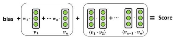 (a) Factorization Machine 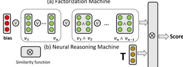 Figure 1: An overview of the fundamental structure of (a) Factorization Machine and (b) Neural Reasoning Machine. As we can see, FM has three components: bias term, first-order features and second-order feature interactions, and it adds up the scores from the three components to calculate the final ranking score, while NRM considers first-order and second-order logical interactions between features, which enables the model to learn the compositional relationships between features for recommendation. Recommender Systems (RS) play an important role on the modern web as well as in many intelligent information systems. They connect users and information by predicting the potential interest of users and proactively provide relevant information to users [1-3]. Many of the existing recommendation methods are designed based on the fundamental idea of similarity matching [4-13]. For example, some early Collaborative Filtering (CF) models [4, 5, 7]—which predict a user's future preferences based on their previous records—use manually designed similarity functions such as cosine similarity [4], Pearson correlation [5] or vector inner product [7] to calculate the user-item similarities. More recently, researchers have considered learning-based similarity functions such as neural networks to match users and items [6, 8] based on the user and item embeddings that are learned from various types of information sources such as text [14, 15], image [16] and knowledge graphs [17-19]. Factorization Machine (FM) [20-23]—as a type of matching-based model that integrates the power of feature-level and user-item-level similarity—unifies the advantages of different matching-based models and achieves better performance in many recommendation tasks. As illustrated in Figure 1(a), FM considers both 1-order and 2-order feature interactions to predict the user-item preference. Researchers further explored FM under the framework of neural similarity matching. One approach is to increase the neural network depth of the feature similarity matching model, such as Deep Factorization Machine (DeepFM) [21] and eXtremely Deep Factorization Machine (xDeepFM) [22], which provided better recommendation accuracy than the original shallow Factorization Machine (FM) model [20]. Other researchers tried to augment the second-order feature interaction from inner-product to neural networks, such as Neural Factorization Machines (NFM) [23], which overcomes the difficulty that FM model cannot learn feature interactions that did not appear in the training set. Due to the generally good performance and the flexibility to incorporate various features, similarity matching-based Factorization Machine models have been widely used in real-world applications [22, 24, 25]. However, as a cognition rather than a perception intelligent task, recommendation not only requires the ability of pattern recognition and matching from data, but also the ability of concrete reasoning in data [26]. This is because users do not make decisions simply based on similar users or items, but they make concrete reasoning about the item features and their relationships to decide the next steps. For example, if a user has already purchased a USB hub, then he or she might purchase a USB drive or an external hard drive instead of purchasing another USB hub in the next step, even though the two USB hubs can be very similar. As a result, if we merely rely on similarity-based models for recommendation, the system might recommend similar products to what the user has already purchased even though the user may not need it any more. In this paper, we propose Neural Reasoning Machine (NRM), which is a neural logical reasoning model for recommendation. NRM is able to learn the conjunction and disjunction relationships between features and items so as to model the compositional nature of the recommendation problem. For example, if a user has already purchased a USB hub, then it's unlikely for the user to purchase another one since the two items are substitutive, which can be represented as a low probability between the conjunction of the two items. Technically, we learn the basic logical operations such as AND $(\land)$, OR $(\lor)$ and NOT $(\neg)$ as neural modules, which are regularized by logical rules to guarantee their logical behavior, and then we represent the feature set of each user-item pair as a logical expression to predict the preference score for the user-item pair, where the logical expression models the logical conjunction and disjunction relationship among the features. For example, if there are two relevant features $v_{1}$ and $v_{2}$ for a user-item pair, then the expression would be $v_{1} \vee v_{2} \vee (v_{1} \wedge v_{2})$, which means that the possible reason for the user to like the item could be feature $v_{1}$, or feature $v_{2}$, or features $v_{1}$ and $v_{2}$ together. We evaluate the probability of truth for the expression to rank the candidate items for recommendation. Experiments on real-world datasets show that our NRM model significantly outperforms traditional matching-based (both shallow and deep) factorization models. The key contribution of this paper are as follow. - We highlight the importance of feature-level reasoning for recommender systems to model the compositional nature of the recommendation problem. - We propose Neural Reasoning Machine (NRM) to integrate symbolic logical reasoning and continuous embedding learning for recommendation. - We conduct both experiments and case studies on several real-world datasets to show the improved recommendation performance and the intuition for such improvements. The following part of the paper will be organized as follows. We review related work in Section 2, introduce details about the model in Section 3, and provide experimental results in Section 4. Finally, conclusions and future work are provided in Section 5. ## II. RELATED WORK Factorization Machine (FM) [20] is one of the most popular types of recommendation models in real-world recommender systems due to their ability to model feature interactions. By embedding all of the features as latent vectors and learning the weight of each vector, FM can estimate the similarity between users and items, and use this as a score to predict the user's preferences on items for recommendation. In addition, FM models the second-order pair-wise interaction between features to improve the prediction accuracy, which is particularly suitable for industry recommender systems which include many features from users and items. Due to the efficiency and flexibility of FM models, they have also been applied to various tasks beyond recommender systems such as stock market prediction [27] and online advertising [28]. Despite that traditional linear FM [20] has been applied to many applications and its effectiveness has been shown to be better than SVM and SVD++ [29] in practice, it still has some important limitations. As a linear model, FM cannot effectively learn and represent nonlinear patterns from data [30, 31]. However, lots of real-world data requires nonlinear pattern recognition and learning, and because traditional FM is limited to linear modeling, FM cannot make satisfactory predictions in such cases. Besides, FM cannot distinguish the importance of different feature interactions. To solve these problems, researchers have made a lot of efforts [22, 32, 33]. For example, Attentional Factorization Machine (AFM) [34] use attention model to specify a proper weight for each feature interaction. Some other research take a different path, which try to integrate deep neural network (DNN) into factorization machine, such as Deep Factorization Machine (DeepFM) [21] and eXtremely Deep Factorization Machine (xDeepFM) [22]. The DeepFM model contains two parts, FM and DNN. The FM part can extract low-order feature information while the DNN part can extract high-order interactive feature information. DeepFM model can learn both low-order and high-order feature information at the same time, without biasing the model to any one side [6, 20]. Compared with DeepFM, xDeepFM model exchanges the FM part in DeepFM with a simple linear network and add a compressed conjunction network (CIN), which further improve the performance of the model. Another solution is Neural Factorization Machines (NFM). Instead of directly inputting the embedding vector into the neural network, NFM builds the Bi-Conjunction operation after the embedding layer. This makes the model be able to learn feature interactions that did not appear in the dataset. Nonlinear networks can bring models with better ability to learn over data and get better prediction accuracy[35]. However, complex real-world scenarios such as online purchase and personalized recommendation not only require the ability of similarity matching from data, but also require the ability of concrete reasoning over the compositional relationships between features and items[26, 36]. This is because users' behaviors are not only driven by the similarity of items, but also driven by users' careful reasoning about what they already have and what they need. Take e-commerce as an example, if a user has already purchased a USB hub, then the user would unlikely purchase another one, but would more likely purchase other products that are compatible with the USB hub, such as a USB drive or an external hard drive. As a result, if we want to recommend products for users in e-commerce websites, we should not simply make recommendations based on the perceptual similarity between items or features, since the probability for a user to buy a substitute in a short time could be low. Instead, we should carefully reason over the compositional (substitutive or complementary) relationships between item features and recommend new items that are compatible with users' previous records. Under this background, researchers have made efforts to integrate logical reasoning and neural networks. For example, traditional approaches such as Markov Logic Networks (MLN)[37-39]integrate probabilistic graphical models with logical reasoning, while more recent Neural Logic Reasoning (NLR)[26, 36]approaches try to integrate logical reasoning and neural networks for intelligent tasks. For example, Neural Logic Reasoning (NLR)[36]builds a logic-integrated neural network (LINN) for solving logical equations and non-personalized recommendation, while Neural Collaborative Reasoning (NCR)[26]models neural Horn clauses for implication reasoning in a latent reasoning space to predict the future preferences of users. (NCR) [26] models neural Horn clauses for implication reasoning in a latent reasoning space to predict the future preferences of users. Although NLR and NCR have shown better recommendation performance based on neural logical reasoning, they are designed to conduct reasoning on user-item interactions rather than reasoning on user or item features. However, many real-world recommender systems need to handle various types of features for recommendation, especially in factorization machine type of models. As a result, we generalize the idea of neural logic reasoning to feature-level reasoning, and propose Neural Reasoning Machine (NRM) to model the compositional relationship between (first-order and higher-order) features for recommendation. ## III. NEURAL REASONING MACHINE We will introduce the details of our Neural Reasoning Machine (NRM) architecture in this section. First, we provide a brief introduction to Factorization Machines (FM) for better comparison between reasoning machine and factorization machine. We then introduce how to construct the reasoning machine based on logical expressions as well as logical regularizers. Finally, we introduce how to learn and optimize the model. ### a) Preliminaries To provide a better comparison between reasoning machine and factorization machine, we first briefly review factorization machine. FM mainly solves the feature interaction problem under sparse data. FM is a linear model, but it still has good generality for both continuous and discrete features. In traditional linear models such as linear regression, we consider each feature individually and do not construct interacted features. However, in many cases, some features combined contain richer and more accurate information than considering each feature individually. For example, a product may be best suitable for male teenagers, as a result, individually considering the gender and age features would not find the best user group for the product, and it is necessary to consider the gender- age interactive feature to solve the problem. For simplicity and efficiency, FM only considers the second-order feature interactions. 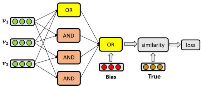 Figure 2: An overview of the connection between the modules in the NRM architecture. The inputs are feature representation vectors. Each pair of feature is conjuncted through the AND module, and then all individual features, conjuncted features as well as the global bias feature are disjuncted through the OR module to build the vector representation for the whole expression, which is compared with the anchor True vector to decide the recommendation score. The model can be represented as. $$ \hat{y}(x) = w_{0} + \sum_{i=1}^{n} w_{i} x_{i} + \sum_{i=1}^{n} \sum_{j=i+1}^{n} w_{ij} x_{i} x_{j} \tag{1} $$ where $x_{i}$ is example $x$ 's value on the i-the feature, which is usually a binary value (1 for triggering the feature and 0 otherwise). The multiplication $x_{i}x_{j}$ represents the interactive feature constructed by $x_{i}$ and $x_{j}$ and this feature is triggered (i.e., value equals 1) if and only if both $x_{i}$ and $x_{j}$ are triggered. Most of the real-world recommendation datasets are very sparse due to the very large amount of users, items and features. As a result, usually only a few of the feature values $x_{i}$ or interactive feature values $x_{i}x_{j}$ are non-zero. Because of the sparse training data and the huge number of interactive feature weight parameters wij to be learned, it is usually impractical to directly train the interactive feature weight matrix $W = [w_{ij}]_{n\times n}$. To solve the problem, we usually use matrix factorization for dimension reduction to parameterize the weight matrix, which gives the following FM formula: $$ \hat {y} (x) = w _ {0} + \sum_ {i = 1} ^ {n} w _ {i} x _ {i} + \sum_ {i = 1} ^ {n} \sum_ {j = i + 1} ^ {n} \langle \mathbf {v} _ {i}, \mathbf {v} _ {j} \rangle x _ {i} x _ {j} \qquad (2) $$ where each feature $i$ is learned as a $k$ -dimension vector representation $\mathbf{v}_i \in \mathbb{R}^k$ and the inner product between two feature vectors denote the importance of this feature combination: $$ \langle \mathbf{v}_i, \mathbf{v}_j \rangle = \sum_{n=1}^{k} v_{i,n} v_{j,n} \tag{3} $$ Eventually, the parameters to be learned in FM include the global bias term w0, the weights of first-order features $\mathbf{w} \in \mathbb{R}^n$ and the vector representation for each feature $\mathbf{v}_i \in \mathbb{R}^k (i = 1,2,\dots,n)$. ### b) The NRM Framework Different from FM which adopts linear addition to combine the influence of (individual and interactive) features, NRM models the compositional logical relationship between features for recommendation. As shown in Figure 2, NRM has three logical modules: AND (A), OR (V) and NOT (¬). NRM employs these three logical modules over the feature vectors and represent each data sample as a logical expression. Mathematically, this can be formulated as: $$ \hat {\mathbf {y}} (x) = \mathbf {v} _ {0} \vee \left(\bigvee_ {i = 1} ^ {n} x _ {i} \mathbf {v} _ {i}\right) \vee \left(\bigvee_ {i = 1} ^ {n} \bigvee_ {j = i + 1} ^ {n} x _ {i} x _ {j} (\mathbf {v} _ {i} \wedge \mathbf {v} _ {j})\right) \tag {4} $$ where $\mathsf{v}_0$ is a global bias vector, $\mathsf{v}_i$ and $\mathsf{v}_j$ are the embedding vectors of the $i$ -th and $j$ -th feature, while $x_i$ and $x_j$ represent the binary values of the two features, e.g., $x_i = 1$ means this data sample triggers feature $i$, and 0 otherwise. As a result, only those triggered individual features (i.e., $x_i = 1$ ) or interactive features (i.e., $x_j x_j = 1$ ) will be considered in the equation. The parameters to be learned in the NRM model include the global vector $\mathsf{v}_0$, each feature's representation vector $\mathsf{v}_i$ ( $i = 1,2, \dots, n$ ), as well as the parameters in the logical modules. The intuition behind the NRM modeling is that: the reason for a user to like or dislike a particular item could be the global feature, OR each of the individual feature, OR each combination (AND) of two features. Comparing Eq. (2) and Eq. (4), the advantage of NRM is its ability to model the compositional relationship between features or feature combinations. More specifically, traditional FM is additive, while NRM is disjunctive, which makes the model more sensitive to good features (or feature combinations) even if such good features (or combinations) are few. Due to the nature of the mathematical OR operation, even one strong signal from a very positive feature can lead to strong predictions. One thing to note is that different from FM whose direct output is a scalar value (Eq.(2)), the direct output of NRM is a vector $\hat{\mathbf{y}} (\mathbf{x})$ (Eq.(4)), which is the vector representation of the data sample corresponding to a user-item pair. To get the final recommendation score, we need to evaluate to what extent $\hat{\mathbf{y}} (\mathbf{x})$ is close to the constant true vector $T$ in the logical reasoning space. Besides, to guarantee that the AND, OR and NOT modules are really conducting the expected logical operations in the reasoning space, we need to apply logical regularization over the modules. We will introduce these techniques in the following subsection. ### c) NRM Expression Calculation ## i. Logical Operators and Anchor Vectors Inspired by Neural Collaborative Reasoning (NCR) [26], we use three independent Multi-Layer Perception (MLP) neural networks to represent the logical operators AND(·, ·), OR(·, ·) and NOT(·). Both AND and OR operators are binary operators, which take two vectors as input and output another vector. The NOT operator is a unitary operator which takes one vector as input and outputs another vector. The answer of a logical expression should be true or false. As a result, we need two anchor vectors which correspond to the constant True and False vector in the reasoning space. The true vector $(T)$ is a randomly initialized vector and once it is initialized, it keeps as a constant vector and never gets updated during the entire training and evaluation process. The false vector $(F)$ is calculated based on the true vector (i.e., $F = \text{NOT}(T)$ ). For example, if the label of an example is positive, we expect that the vector representation of the corresponding logical expression should be close to the true vector $(T)$, otherwise, if the label is negative, we expect the vector representation would be far away from the true vector and close to the false vector $(F)$. ## ii. Calculate Logical Expression With these logical modules and anchor vectors, we can calculate the vector representation of the logical expression in NRM. The initial input to NRM are the user or item features of an example. Suppose an example includes two features $v_{1}$ and $v_{2}$ (i.e., $x_{1} = x_{2} = 1$ ). The output vector of OR $(v_{1}, v_{2})$ represents that the user may like the item because of feature $v_{1}$ or feature $v_{2}$, while AND $(v_{1}, v_{2})$ can represent the possible reason of feature $v_{1}$ and $v_{2}$ together. Combined with the feature values $(x_{i})$ and bias vector $(v_{0})$, we can get the final expression of this example: $$ \hat {\mathbf {y}} = \mathbf {v} _ {0} \vee (x _ {1} \mathbf {v} _ {1} \vee x _ {2} \mathbf {v} _ {2}) \vee (x _ {1} x _ {2} \mathbf {v} _ {1} \wedge \mathbf {v} _ {2}) \tag {5} $$ When we get the output vector representation $\hat{\mathbf{y}}$, the next step is to decide whether the logical expression is true or false. To achieve this goal, we need to compare the vector $\hat{\mathbf{y}}$ and the anchored vector $T$. As we mentioned before, if the example is positive, then the representation vector $\hat{\mathbf{y}}$ should be close to the $T$ vector. Otherwise, it should be away from the $T$ vector. In this work, we use the cosine similarity function to compare the vector representation $\hat{\mathbf{y}}$ of an expression with the $T$ vector. $$ \operatorname{Sim} (\hat{\mathbf{y}}, T) = \frac{\hat{\mathbf{y}} \cdot T}{\| \hat{\mathbf{y}} \| \| T \|} \tag{6} $$ To ensure that the logical modules such as AND and OR perform the corresponding logical operations as expected, we add logical regularizers to the neural modules to regularize their behavior. For example, the following logical regularizer is added to the OR module to make sure the operator satisfies the Annihilator law, e.g., $v \lor T = T$: $$ r = \frac{1}{\chi} \sum_ {\upsilon \in \chi} 1 - \operatorname{Sim} (\operatorname{O R} (\mathbf{v}, \mathbf{T}), \mathbf{T}) \tag{7} $$ where $\mathsf{v}$ is the corresponding vector of a variable, $\chi$ represents the variable space, Sim $(\cdot,\cdot)$ represents the similarity function, which is cosine similarity in this work. Intuitively, by minimizing this regularizer, the model makes sure that $\upsilon \vee T$ is close to $T$. Details of the many other logical regularizers are similar as [26, 36]. We not only apply regularizers to the input embedding vectors but also to the intermediate latent vectors to ensure that all vectors are in the same representation space and follow the same constraints. Take the logical expression in Eq. (5) as an example, we will add regularizers to $\mathsf{v}_0,\mathsf{v}_1,\mathsf{v}_2$, as well as the output vectors of $(\mathsf{v}_1\vee \mathsf{v}_2)$ and $(\mathsf{v}_1\wedge \mathsf{v}_2)$. The logic constraint loss is represented as $L_{r}$, which represents the sum of all of the logical regularizers. It will be added to the training loss in the learning process. ### d) Final Loss and Learning Method The final prediction of NRM is the output of the similarity function (Eq. (6)). The range of the cosine similarity function is - 1 to 1, however, the label of our dataset set is 0 and 1. To make the output of NRM compatible with the label, we amplify the cosine similarity output in Eq.(6) by $\zeta$ and pass the value through a sigmoid function: $$ \hat{y} = \sigma (\zeta \cdot \operatorname{Sim} (\hat{\mathbf{y}}, \mathbf{T})) \tag{8} $$ where $\sigma (\cdot)$ is the sigmoid function, $\zeta$ is the coefficient to amplify the output of similarity function. Then we calculate the square error to estimate the difference between the prediction and the label: $$ L o s s = (\hat {y} - y) ^ {2} \tag {9} $$ where $\hat{y}$ is the prediction of NRM and $y$ is the ground-truth label. At the same time, we calculate the logical regularizer. $$ L _ {r} = \gamma \sum_ {i} r _ {i} \tag {10} $$ where each $r_i$ represents a logical regularizer as in [26, 36], and $\gamma$ is the coefficient of the logical regularizer. Logical constraints help the NRM model to achieve better performance, but we need to balance the weight between the logical constraint and the prediction loss by $\gamma$. In the experiment section, we will study how the coefficient influences the experimental result. We sum up the logical regularizer and the prediction loss as the final loss function. Then the model minimizes the loss to optimize the model parameters. $$ Loss = \sum_{x \in \mathcal{D}} (\hat{y} - y)^{2} + L_{r} $$ where $\mathcal{D}$ is the set of training samples. We will introduce the experimental settings and explore the recommendation performance of NRM in the following section. ## IV. EXPERIMENT In this section, we conduct experiments in three real-world datasets and compare the results of NRM and baselines to verify the effectiveness of our model. We aim to answer the following research questions: - RQ1: What is the performance of NRM in terms of hit ratio and NDCG? Does it achieve better result than state-of-the-art factorization machine models? - RQ2: How does the logical regularizer help to improve the performance? - RQ3: What is the impact of the conjunction part of the model? ### a) Dataset We use three real-world datasets in the experiments. We introduce the details about the datasets in the following. - MovieLens100K \[40\]: This is a frequently used dataset maintained by Grouplens. The MovieLens dataset was first released in 1998 and has become popular since the publication. Many research have adopted this database. This dataset describes users' expressed preferences for movies. The dataset keeps updating, and we use the latest version released by Grouplens. It contains 100,000 movie ratings ranging from 1 to 5 from 610 users to 9724 movies. - Amazon \[41\]: This is the Amazon e-commerce dataset, which includes user, item and rating information spanning from May 1996 to Oct 2018. This dataset is an updated version of the Amazon review dataset released in 2014. This is also a frequently used dataset adopted by many research. It contains 24 different categories as sub-datasets. We use two very different categories Grocery and Electronics to explore the performance of our model under different product recommendation scenarios. Table 1: Basic Statistics of the Datasets <table><tr><td>Dataset</td><td>#users</td><td>#items</td><td>#features</td><td>#instance</td></tr><tr><td>MovieLens 100K</td><td>610</td><td>9724</td><td>10334</td><td>100000</td></tr><tr><td>Grocery</td><td>854</td><td>14700</td><td>15554</td><td>45575</td></tr><tr><td>Electronics</td><td>16530</td><td>65848</td><td>82376</td><td>446367</td></tr></table> Some basic statistics of the datasets are shown in Table 1. Because some of the baselines need explicit feedback, for fair comparison, for all of the models in this paper, we all use explicit feedback datasets. The original dataset contains rating information. We use this information as explicit feedback. Following common practice, we consider 1-3 ratings as negative feedback and 4-5 ratings as positive feedback. According to the suggestions of [42], we use leave-one-out setting to split the training set, validation set and testing set. To avoid data leakage, for each user, we put the user's most recent two positive interactions into the validation set and testing set, respectively, and put the rest interactions into the training set. All of the baselines and NRM use the same data to make sure the experiment is fair and models are comparable. ### b) Baselines In this section, we make a brief introduction to the baselines used in the experiments. We compare with five baseline models. Three of the five baselines do not have open-source implementation, so we implemented them by PyTorch, an open-source deep learning library. The baselines have open-source implementations[^1], and thus we directly use the open-source implementation for experiments. For anonymity, we will publicize our code later. - FM: Factorization Machines (FM) mainly solves the problem of feature interaction under sparse data. Its prediction complexity is linear, and it has good generality for continuous and discrete features. We consider FM as a baseline of our model because FM is a fundamental and widely used factorization model. - NFM: Neural Factorization Machine (NFM) introduces Bi-linear Interaction (Bi-Interaction) pooling operation in neural networks. Based on this, the model can learn combined features that do not appear in the dataset, which helps to better learn and predict in real-world data. - DeepFM: Deep Factorization Machine (DeepFM) combines deep neural networks and FM. It constructs a Multi-Layer Perception (MLP) to learn the embedding features. - xDeepFM: eXtremely Deep Factorization Machine (xDeepFM) purposes a Compressed Conjunction Network (CIN), which compresses the pairwise feature interaction matrix into one dimension. Different from DeepFM, xDeepFM learns specific weights for the linear layer, deep learning layer and CIN during the training process. - NCR: Neural Collaborative Reasoning (NCR) is the state-of-the-art neural reasoning model for recommendation. It represents users' behavior over items as a logical expression. By learning these logical expressions, NCR can predict users' future behaviors. The difference between NCR and our model is that NCR conducts reasoning on item-level while our model conducts reasoning on feature-level. recommendation. It represents users' behavior over items as a logical expression. By learning these logical expressions, NCR can predict users' future behaviors. The difference between NCR and our model is that NCR conducts reasoning on item-level while our model conducts reasoning on feature-level. Table 2: Experimental results on Hit Ratio (HR) and Normalize Discounted cumulative gain (NDCG). Bold numbers represent better performance. We use star (\*) to indicate that the performance is significantly better than all baselines. The significance is at 0.05 level based on paired t-test. <table><tr><td>Dataset</td><td colspan="4">ML100K</td><td colspan="4">Grocery</td><td colspan="4">Electronics</td></tr><tr><td>Metric</td><td>NDCG@10</td><td>NDCG@5</td><td>Hit@10</td><td>Hit@5</td><td>NDCG@10</td><td>NDCG@5</td><td>Hit@10</td><td>Hit@5</td><td>NDCG@10</td><td>NDCG@5</td><td>Hit@10</td><td>Hit@5</td></tr><tr><td>FM</td><td>0.169</td><td>0.128</td><td>0.328</td><td>0.202</td><td>0.057</td><td>0.045</td><td>0.109</td><td>0.072</td><td>0.056</td><td>0.038</td><td>0.117</td><td>0.062</td></tr><tr><td>NFM</td><td>0.212</td><td>0.182</td><td>0.361</td><td>0.271</td><td>0.085</td><td>0.061</td><td>0.183</td><td>0.108</td><td>0.057</td><td>0.045</td><td>0.109</td><td>0.072</td></tr><tr><td>DeepFM</td><td>0.197</td><td>0.160</td><td>0.351</td><td>0.236</td><td>0.068</td><td>0.052</td><td>0.133</td><td>0.081</td><td>0.061</td><td>0.043</td><td>0.127</td><td>0.070</td></tr><tr><td>xDeepFM</td><td>0.159</td><td>0.131</td><td>0.283</td><td>0.198</td><td>0.072</td><td>0.058</td><td>0.202</td><td>0.126</td><td>0.177</td><td>0.146</td><td>0.311</td><td>0.213</td></tr><tr><td>NCR</td><td>0.184</td><td>0.146</td><td>0.329</td><td>0.218</td><td>0.182</td><td>0.161</td><td>0.334</td><td>0.248</td><td>0.142</td><td>0.126</td><td>0.273</td><td>0.192</td></tr><tr><td>NRM</td><td>0.226*</td><td>0.186</td><td>0.419*</td><td>0.296*</td><td>0.203*</td><td>0.162</td><td>0.381*</td><td>0.255</td><td>0.189*</td><td>0.159*</td><td>0.320*</td><td>0.231*</td></tr></table> ### c) Parameter Settings The learning rate was searched in [0.001; 0.01; 0.02; 0.05] for all methods. We apply ReLU non-linear as activation function between logical operations. For all models, we make the feature embedding size as 128, the batch size is 4096. We run 20 epochs and record the best result. For fair comparison, for all models, including our model and baselines, we tune each model's parameter to its own best performance on the validation set. All experiments were conducted on a single NVIDIA GeForce 2080Ti GPU. The operating system is Ubuntu 16.04 LTS. ### d) Evaluation Metric For each user-item pair in the testing and validation set, we randomly sample 99 irrelevant features to exchange the first item feature of the user-item pair. And we use these 100 user-item pairs for evaluation. The model that has a better performance should get a higher score for the true user-item pair than others. We use Hit Ratio (H R) and Normalize Discounted Cumulative Gain (NDCG) to evaluate the models. HR is used to measure whether the correct item appears in the top-K list. DCG is accumulated from the top of the result list to the bottom, with the gain of each result discounted at lower ranks [43]. NDCG is the ratio between DCG and the Idealized Discounted Cumulative Gain (IDCG). These two metrics are widely used in recommendation system evaluation [44, 45]. For HR and NDCG, larger value means better performance. ### e) Performance Comparison The experimental results on Hit Ratio (HR), and Normalize Discounted Cumulative Gain (NDCG) are shown on Table 2. Based on the experiment results, we have following observations. First and most importantly, compared with the five baselines in most cases, our NRM model achieves significantly better performance than the baselines on all of the three datasets. Although NRM is only slightly better than the best baseline in a few cases, e.g., on ML100K the NDCG@5 of NRM is slightly better than NFM (0.186 vs 0.182), however, in 9 out of 12 cases, our NRM model has a significant improvement against the best performance in baselines. For example, on ML100K the Hit@10 result of NRM is 0.419 while the best result of the baselines is 0.361, and the improvement from the best baseline result is $16.06\%$. The reason why NRM can get better result is that linear models such as FM suffers from learning nonlinear real-world data. When faces with complex scenarios, these models will encounter some problems. For example, these models will recommend the user a substitute of the item that the user purchased recently. Previous neural logical models, like NCR, lacks of the information of second-order feature interactions. NRM draws on the advantages of these models and improves on their shortcomings. Neural logical modules in NRM bring the model ability to find the relationship between features in the user-item pair. Thus NRM can predict the user's future behaviors more accurately. Compared to NCR, our model has second-order feature interactions, which can help the model find latent information in these feature interactions. Compared to the Amazon dataset, most models have a better results on MovieLens 100K. This is because MovieLens 100K is more dense than Amazon dataset. For MovieLens 100K, it has less users, more items and more instances, which means for each user, MovieLens 100K has more items and history information. And this will make the models much easier to analyse the user's behavior pattern and predict the user's future behaviors. We also conduct some qualitative analysis of the product ranking results, as shown in Table 3. First, for the same product recommendation, we see that the correct prediction gains a higher rank in our NRM model. Second, compared to the baseline models, the top-10 ranked products recommended by our NRM model tend to be more relevant to the given purchase history and more similar to the correct prediction. As shown on Table 3, the user bought three products recently: a USB high speed hub, audio cable and speaker. Based on these three products our NRM model recommends more related products instead of similar products, such as external hard drive and memory card reader. While the other three models recommend some products that the user has bought recently, such as USB hub and speakers. There is only a little possibility for the user to buy the same kind of products in such a short period of time. This is because these models only consider the similarity between the prediction products and recently purchased products. While for our NRM model, the logical modules and logical regularizers make the model will consider not only the similarity but also the relationship between these products. Therefore, our model has natural advantages in those complex real-world scenarios where only similarity matching cannot satisfy. Table 3: Qualitative Results on Ranking. Bold Items are the Ground Truth or Substitutes of the Ground Truth. We Use Star (\*) to Indicate the Ground Truth. Items Have the Same Genres with Latest Purchased Items are in Strike through to Highlight the Difference Items <table><tr><td>Dataset</td><td colspan="4">Amazon Electronics</td></tr><tr><td>Ground Truth</td><td colspan="4">USB flash drive</td></tr><tr><td>Latest three items</td><td colspan="4">USB High Speed Hub/Audio Cable/Speakers</td></tr><tr><td>Model</td><td>FM</td><td>NFM</td><td>DeepFM</td><td>NRM</td></tr><tr><td rowspan="10">Predicted Top-10 Products</td><td>TV</td><td>Headset</td><td>Tripod</td><td>External Hard drive</td></tr><tr><td>SD Card</td><td>Media Player</td><td>computer case</td><td>USB flash drive*</td></tr><tr><td>USB-Hub</td><td>USB-Hub</td><td>Hard Drive Case</td><td>Tripod</td></tr><tr><td>Speakers</td><td>External Battery</td><td>Network Router</td><td>External Battery</td></tr><tr><td>Desktop Memory</td><td>Flash Memory Card</td><td>Solid State Drive</td><td>Headset</td></tr><tr><td>USB Mouse</td><td>Microfiber Cleaning Cloths</td><td>Phone Camera Lens</td><td>computer case</td></tr><tr><td>Media Player</td><td>USB flash drive*</td><td>Bag for Headset</td><td>Memory Card Reader</td></tr><tr><td>Ethernet Adapter</td><td>Memory Card Reader</td><td>USB flash drive*</td><td>Media Player</td></tr><tr><td>External Hard Drive</td><td>Speakers</td><td>Speakers</td><td>USB flash drive</td></tr><tr><td>Antenna Mount</td><td>MacBook Pro</td><td>Audio Cable</td><td>External Battery</td></tr></table>   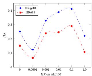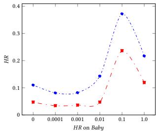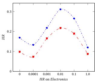 Figure 3: Performance on Hit Ratio on Different Regularizer Coefficient with Different Datasets ### f) Impact of Logical Constraint In this section, we answer the question about how the logical regularizer help the learning process. In the experiments, we set regularizer coefficient in [0, 0.0001, 0.001, 0.01, 0.1, 1.0] for ML100K, Grocery and Gourmet Food and Electronic. And we show the experiment results HR@10 and HR@5 in Figure 3. The results show that the logical regularizers do help to improve the performance of NRM. When we compare the results of the non-logical regularizer model $(\gamma = 0)$ with the logical regularizer model $(\gamma \neq 0)$, we can find the results with the logical regularizer are better. However, the logical regularizers coefficient should be adjusted very carefully. Otherwise, the model might have even worse performance than the non-logical regularizer model. Overall, for all of these three datasets, the best logical regularizer coefficient is around 0.01 and 0.1. If the coefficient is bigger than this, the performance will become worse. This is because there is a trade off between prediction loss and logical constraint loss. If the coefficient is too big, logical constraint loss will dominate the loss, and the model will only learn limited information from the data. Therefore we need to balance the weight between prediction loss and logical constraint loss to make sure the model can learn useful information from both of them. ### g) Impact of Conjunction Part In this section, we answer how the conjunction part in the NRM model helps the learning process. In the experiments, we omit the conjunction part in the NRM model and make comparison with the normal NRM model with conjunction part. We show the NDCG@10, NDCG@5, Hit@10 and Hit@5 results in Figure 4. Compared to the NRM without conjunction part, the normal NRM model has better performance on all of the datasets. In the conjunction part, NRM learn information from second-order feature interactions and help the model make more accurate prediction. If we do not consider the conjunction part, the performance will have a significant decrease. This is because only first-order feature interactions are not sufficient for NRM to learn the relationship between different features. As a result, the performance will become much worse than the normal NRM model that has a conjunction part.   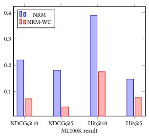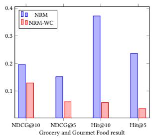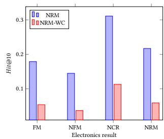 Figure 4: Performance on NRM and NRM without Conjunction Part. The Blue Bar is the Results for NRM and the Red Bar is the Results for NRM without Conjunction (NRM-WC) Part ## V. CONCLUSION AND FUTURE WORK In this paper, we propose a Neural Reasoning Machine (NRM), which integrates neural logical modules and recommendation task. What's more, our NRM model have a better performance than the state-of-the-art baseline. Experiments on three real world datasets have shown the potential of NRM in practice. This is just the beginning of our work. There are some other methods, such as [26, 46], that have been proved to be effective on the recommendation. However, their limited expressive ability may limit the model's learning of latent information behind real-world data. By introducing neural logic modules, the learning ability of these models can be further improved. With the recent development of technology, it is not very hard to construct an extreme deep neural network [47, 48]. However, a deeper neural network means more running time of generating and optimizing the model, and this does not always come with good results [49]. Therefore, for future works, we would like to focus more on how to design better neural components or architectures for specific tasks. Other than the recommendation systems, we expect the idea of neural reasoning can be used in more fields such as Computer Vision, Natural Language Processing, Graph Neural Network and Social Network. In these fields, logical reasoning is also a very important part, which will make the result more reliable and explainable. CCS Concepts Information systems $\rightarrow$ Recommender systems; Computing methodologies $\rightarrow$ Machine learning. [^1]: https://github.com/rixwew/pytorch-fm _(p.6)_

Generating HTML Viewer...

References

40 Cites in Article
Huifeng Guo,Ruiming Tang,Yunming Ye,Zhenguo Li,Xiuqiang He (2017). DeepFM: A Factorization-Machine based Neural Network for CTR Prediction.
Jianxun Lian,Xiaohuan Zhou,Fuzheng Zhang,Zhongxia Chen,Xing Xie,Guangzhong Sun (2018). xdeepfm: Combining explicit and implicit feature interac-tions for recommender systems.
Explore published articles in an immersive Augmented Reality environment. Our platform converts research papers into interactive 3D books, allowing readers to view and interact with content using AR and VR compatible devices.
Your published article is automatically converted into a realistic 3D book. Flip through pages and read research papers in a more engaging and interactive format.
Most of the existing recommendation models are designed based on the principles of learning and matching: by learning the user and item embeddings and using learned or designed functions as matching models, they try to explore the similarity pattern between users and items for recommendation. However, recommendation is not only a perceptual matching task, but also a cognitive reasoning task because user behaviors are not merely based on item similarity but also based on users’ careful reasoning about what they need and what they want.
Our website is actively being updated, and changes may occur frequently. Please clear your browser cache if needed. For feedback or error reporting, please email [email protected]
Thank you for connecting with us. We will respond to you shortly.