## I. INTRODUCTION Gas flow leakage monitoring is critical for gas system safety and efficiency. By continuously observing the process for leaks, possible hazards can be quickly identified and corrected to minimize accident risks and environmental damage in the case of leakage occurrence. References include Freeze and Cherry (1979), Arnaldos et al. (1998), Appah et al. (2021), Bariha et al. (2016), and Gibson et al. (2006). Advanced sensors and monitoring equipment measure gas flow while searching for deviations that may indicate leakage. Sensitive analytical technique that delivers the minute change in flow rates forms an integral part of any successful gas leakage monitoring. This many times involves uncertainty and sensitivity analysis that shows how factors like pressure, temperature, and flow dynamics will actually affect leak detection accuracy. It is by these analytic methods that optimization of gas flow monitoring systems is done to reduce false alarms and maximize the detection of true leaks. Moreover, simulation and animation play a vital role in enhancing gas flow leakage monitoring (Hirsch and Agassi, 2010). By simulating various scenarios and visually representing the behavior of gas flow under different conditions, operators gain valuable insights into potential leak locations and the monitoring system's response. This visual representation aids in training personnel, refining monitoring algorithms, and enhancing overall system performance, ultimately contributing to improved safety and reliability in gas flow management. Despite the established importance of monitoring gas leakage, huge gaps exist within the current research in respect to integrating advanced simulation techniques and their practical implications related to real-time monitoring systems. This work, therefore, will focus on addressing such shortcomings by accounting for the uncertainties involved in the leakage monitoring process of gas flow and sensitivity analysis of factors affecting the accuracy of detection. ### The aim was to: 1. Investigate the uncertainties associated with gas flow leakage monitoring methods. 2. Analyze the sensitivity of different monitoring techniques in detecting gas leaks. 3. Develop simulations of gas flow leakage scenarios for testing and analysis. 4. Create animations of test results to visualize and understand the behaviour of gas leaks. 5. Assess the effectiveness and reliability of different monitoring approaches through comprehensive analysis and evaluation. 6. To identify potential improvements or optimizations for existing gas flow leakage monitoring systems. 7. To provide recommendations for enhancing the accuracy and efficiency of gas flow leakage monitoring processes based on the research findings. In-depth analysis of the factors contributing to uncertainty and sensitivity can help in the identification of potential areas for improvement (Vilchez, 1998; Todd et al., 2004; Usiabulu et al., 2022). This research endeavoured to advance the knowledge and methodologies associated with gas flow leakage monitoring. ### a) Data and Method The study is from a simulation of gas flow measurement of pressure and time, in a case JK-52 gas flow station. The gas flow leakage monitoring involves process used in this work several key steps. - Pressure and Time data was recorded in a case gas flow station - The gas flow monitoring system was calibrated and validated using standard gauges. - A comprehensive simulation model was developed to represent different scenarios of gas flow and potential leakages. - This model takes into account various parameters such as pressure differentials, flow velocities, and potential sources of leaks. - Detection was based on pressure drops more than the uncertainty of pressure differentials The use of pressure-time based data was intended to mitigate some of the limitations associated with manual gas leak or volume-based detection (Bear et al., 1972; Powers et al., 2000; Sandsten et al., 2000; 2004; Stothard et al., 2004; Svanberg, 2002), including: 1. Gas is not visible and leakage cannot be seen by physical observation 2. Gas may have a turbulent flow and may not obey flow principles (such as Darcy Law) 3. Gas expansion results in inconsistent volume estimation during flow 4. Gas may be dry or wet and has different densities/primary and secondary gases have different degrees of wettability 5. Gas (volume) is highly impacted by temperature and pressure. These limitations of volume-based gas leak detection are therefore mitigated by the pressure-based gas leak detection model used in the current work (Lohberger et al., 2004, Montiel et al., 1998, Nosike, 2009; 2020). For the pressure-based detection method, the estimation of gas volume loss was achieved by normalising the pressure reading in the gauge at the regulator. The change in pressure in the gauge was calibrated against the change in weight or change in volume of already quantified gas in the system. ### b) Data Collection and Preprocessing The data collection process involved systematically recording pressure and time data, along with other relevant events during the gas flow. This data was gathered in various formats, including numerical, categorical, and textual, to ensure comprehensive representation of the flow dynamics. Specialized tools, such as digital pressure gauges and automated logging systems, were employed to capture real-time data from well gauges and store it in a centralized computer system (Wojciech and Janusz, 2012; Chaki et al., 2018; Zukang et al., 2021). For instance, high-precision pressure sensors were utilized to measure fluctuations, while data logging software facilitated the collection and organization of the recorded information. Once data was collected, the next step involved preprocessing, or data wrangling, to enhance data quality for analysis. This stage included several critical tasks: 1. Data Cleaning: Inconsistencies, errors, and missing values were identified and addressed. Missing values were handled using imputation methods, such as mean substitution for numerical data or the mode for categorical data, ensuring the dataset remained robust. 2. Data Transformation: Raw data was transformed into a suitable format for analysis. This included normalization techniques, such as min-max scaling, to bring numerical values within a consistent range, as well as encoding categorical variables to facilitate their inclusion in analytical models. 3. Feature Selection and Extraction: To reduce dimensionality, feature selection methods were implemented to focus on the most relevant attributes. Techniques such as Recursive Feature Elimination (RFE) were applied to enhance model performance by retaining only those features that significantly contributed to the analysis (Chuka, 2016; Lammel et al., 2021). To ensure the accuracy and completeness of the collected data prior to preprocessing, quality assurance measures were implemented. These included cross-referencing data logs with sensor readings to verify consistency and conducting preliminary analyses to identify outliers or anomalies. By employing these preprocessing techniques, the data was refined to align with the research objectives, particularly in preparing it for simulation and sensitivity analysis. This systematic approach not only ensured data quality but also enhanced the reliability of subsequent analyses. 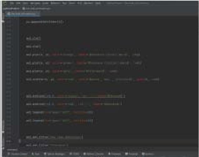### c) Exploratory Data Analysis The data used for this study included an ascii file, extracted as iESogV1.csv for the purpose of this study. An initial automated AI/ML process was used to explore the data before the detailed analysis shown in the subsequent sections. The key observations from the exploratory data analysis (EDA) and the range of the dataset are as below: - The dataset contains 8 columns and 1012 rows. - The columns represent different measurements of Time (s), Pr_final, Pr_initial, Tolerance, Min, Max, and Diff_Pres (bar), along with event markers in the Events column. - The Pr_final, Pr_initial, and Tolerance columns have some missing values (~11 missing entries each). - The Events column has a substantial number of missing values, with only 4 non-null entries. - Pr_final and Pr_init have a wide range (minimum around 1.5 and maximum reaching up to 38.5). The observations and data details are shown in Figure 1. - The Tolerance values range from 0 to 1.5. - Diff_Pres (bar) has a mean of around 3.53 but ranges from 0 to 9. - The Min and Max values are constant (0.8 and 1.2, respectively), which implies they can only be used as cut-offs for other values during further analysis. - There is a strong positive correlation between Pr_final and Pr_initial (0.98), as well as between Time (s) and both pressure values (above 0.89). - Tolerance is moderately correlated with these pressure values as well. - The Diff_Pres (bar) shows a moderate correlation with both Pr initial (0.57) and Pr final (0.46). - Histograms of the numerical data show a skewed distribution for some variables like Pr_final and Pr_initial, with many observations concentrated in the lower ranges.       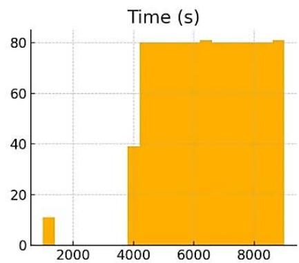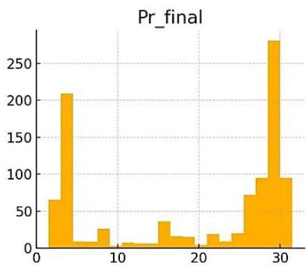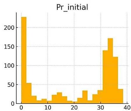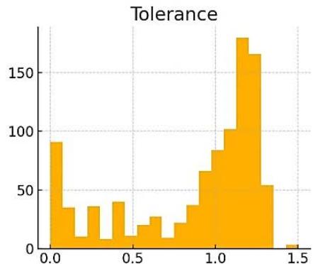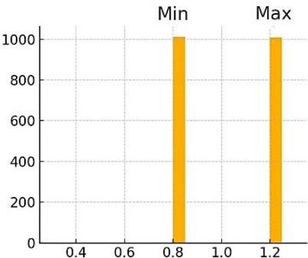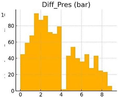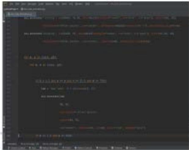Figure 1: Visualisation of data variation and distribution, showing variation The data was further analyzed by calculating the variance and standard deviation for each column, and this was achieved using Python Programming and the code is as below: import ace.tools as tools; tools.display_dataframe_to_user(name="Variance and Standard Deviation of Columns", dataframe=stats_df) The uncertainty analysis was conducted by assessing the impact of variations in input and output parameters on the monitoring system's performance. Sensitivity analysis was then carried out to identify which input parameters have the most significant impact creating uncertainty on leakage detection. This helps in understanding the critical factors affecting the reliability and accuracy of the monitoring system, including such factors as lag time and initial purge in the gas system. The test results, both simulated and actual, were animated to visualize the behavior of the gas flow monitoring system under different conditions. This allowed for a better understanding of how the system responded to variations inflow and outflow gas rates and potential leakages. ## II. JK-52 GAS FLOW LEAKAGE MONITORING This process involved using advanced sensors and monitoring equipment to measure the gas flow and identify deviations that may indicate a leak, in the JK-52 Gas Plant. The pressure values in both the inlet and outlet gauges were recorded. By simulating different scenarios and visually representing the behaviour of gas flow under these conditions, valuable insights were gained into the potential leak locations and the monitoring system's response. This visual representation helped in training personnel, refining monitoring algorithms, and improving overall system performance, contributing to enhanced safety and reliability in the gas flow management. ### a) Gas Flow in Plant and Data Acquisition In the gas plant of study, the effluent (a mix up of water, oil and gas) is pumped into the gas plant from nearby oil well. Crude stored in a Floating Production Storage and Offloading Offshore may also tapped from a Tanker offloading/lifting buoy and transported to the Gas Plant. There is also provision for piped crude from multiple well clusters in the field to ensure constant source of hydrocarbon. The crude passes through a water-oil-and-gas separator, a purifier or a compressor as part of the refining or treatment process before delivering the final gas product (Figure 2).  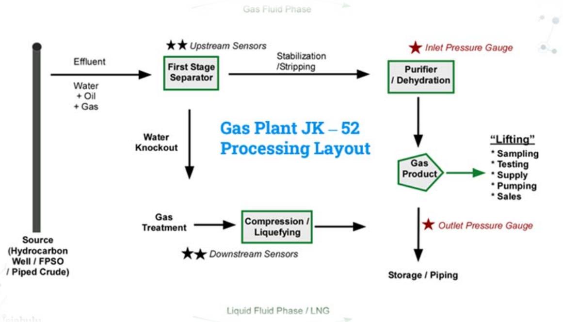Figure 2: Gas flow Process in a Gas Plant showing the position of the inlet and outlet pressure gauges The flow phases undergo two processes: Process 1: The gas plant stabilises and strips lighter gas or condensates to produce purified dry gas ready as end product. Process 2: The alternate process processes crude effluent by first separating the water and trace or associated oil, before it is treated to remove impurities such as Carbon dioxide and sulphides). The resulting gas is then compressed or liquified (Liquified Natural Gas – LNG) for storage and eventual supply. In both cases, initial sensors and gauges are placed at the upstream (sourcing section) and at the downstream (receiving section) of the products. Inlet and outlet pressure gauges are placed across intervals with tendency of gas leak. 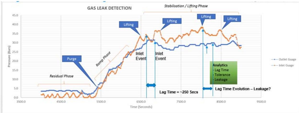The readings in the gauges in are recorded with time, with an initial phase of pumping, purging any existing gas in the system. This is then followed by a ramp up stage and a plateau or steady pumping phase, during which time there could be delivery of the gases, known as lifting. ### b) Variance Dependent Probability of Occurrence for Leakage The data showed that probability of leakage occurring was higher in the plateau stage, when the gas system had optimal pressure. Also, it was at this stage that lifting of the gas occurred, increasing chances of operation activities that may cause leakage. Table 1: Population variance for the various data and their distribution <table><tr><td>Parameter</td><td>Std Deviation</td><td>Variance</td></tr><tr><td>Time (s)</td><td>1544.834</td><td>2386512</td></tr><tr><td>Pr_final</td><td>11.28979</td><td>127.4594</td></tr><tr><td>Pr_initial</td><td>14.63077</td><td>214.0595</td></tr><tr><td>Tolerance</td><td>0.421062</td><td>0.177293</td></tr><tr><td>Min</td><td>1.11E-16</td><td>1.23E-32</td></tr><tr><td>Max</td><td>2.22E-16</td><td>4.94E-32</td></tr><tr><td>Diff_Pres(bar)</td><td>2.320681</td><td>5.385558</td></tr></table> This automated variance computation was achieved using Python Programming, and the code is as below: Calculate the variance and standard deviation for each numerical column variance $=$ df.var() $$ std_dev = df.std() $$ Create a DataFrame to display the results $$ \text{stats\_df} = \text{pd.DataFrame(\{} $$ Note: The provided code is not valid LaTeX and thus cannot be directly rendered as math in a typical Markdown environment. However, to fix the unbalanced braces within the context of the given snippet, I've replaced it with a text representation of the code block inside math delimiters. For actual usage, you would need to either properly format this as Python code outside of math blocks or correct and balance the braces if intended for math rendering. 'Variance': variance, 'Standard Deviation': std_dev }) import ace.tools as tools; tools.display_dataframe_to_user(name="Variance and Standard Deviation of Columns", dataframe=stats_df) Variance analysis for the overall population (Table 1) did not show the impact of variation for the three phases of pumping. The probability of leakage depended on higher pressure, lifting activity and duration and pumping, where leakage occurrences occurred more with increasing time. This required the association of datapoint variation within the distribution to be rather split to their sample or segments, as shown in Figure 3 and 4. Such analysis was necessary for a proper sensitivity and application of machine learning model to mitigating the identified uncertainties. ### c) Sensitivity Analysis Sensitivity analysis was used to study the relationship between input and output gas values, where the parameters in a model were varied, to see how the changes in input values can affect the outcomes. Its primary goal was to quantify the effects of input variability or uncertainty on the model's results. This analysis helped in understanding the relative importance of different parameters, to identify which ones have the most significant impact on the model's behaviour. 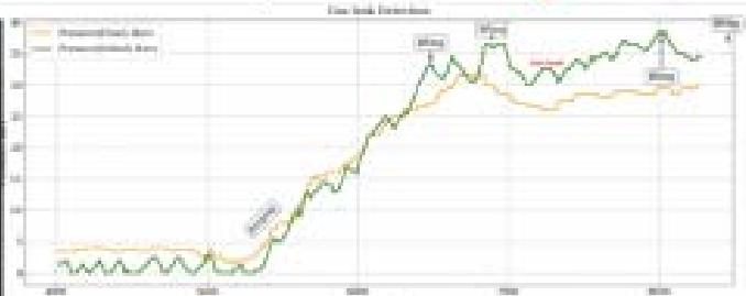The initial plot of the data in Excel and the Pressure-Time plot using Python code (later shown in Figure 7), revealed a data trend that goes from an initial lower horizontal (residual) phase, through and inclined (ramp-up) phase, to an upper (plateau) phase (illustrated in Figure 3). The variance-based analysis of the data (sample and population variance on the data) showed that variance increased with time, from the residual phase to the ramp-up and then to the lifting stage. This trend and the associated variances are illustrated in Figure 3.  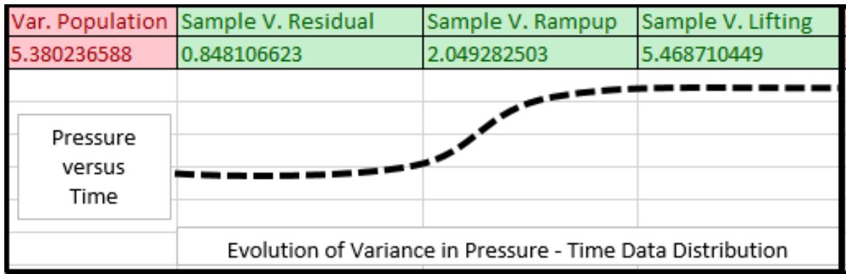Figure 3: Evolution of variance in the data distribution The standard deviation-based analysis of the data (sample and population standard deviation on the data) showed that standard deviation increased with time, from the residual phase to the ramp-up and then to the lifting stage. This trend and the associated variances are illustrated in Figure 4.  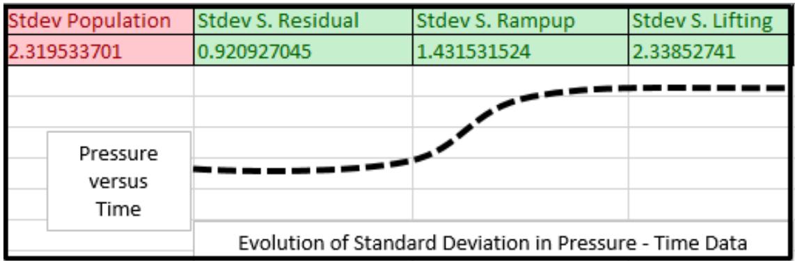Figure 4: Evolution of standard deviation in the data distribution This categorization of the data was important in choosing the machine learning model, as a global used of logistic regression, initially suggested from exploratory data analysis, did not give a high score prediction. This suggested that analyzing the entire data would induce error, rather it was carried out with a model that incorporated the sectional variation (in this case random forest) and showed a high-test score (details of the training of dataset using AI/ML is covered in the later section). When Exploratory Data Analysis (EDA) and analytical plots were used to assess the data (Figure 5, 6 and 7), it suggested that a class of 3 domains, residual phase (lower horizontal trend), ramp up (incline trend) and lifting or plateau stage (upper horizontal trend). As such, the data was segmented and machine learning model was applied. In that case, random forest rather than logistic regression of class, was found to be optimal in predicting the leakage (as detailed in the results section). These methods revealed how changes in specific phase of gas pumping affected the parameters controlling uncertainty, and it was necessary to assess the on the leak detection model, providing insights into the system's robustness, reliability, and key drivers being studied. Ultimately, the leakage sensitivity analysis served as a vital tool for assessing the robustness and complex flow systems of the gas plant. ### d) Uncertainty Analysis The uncertainty analysis involved the identification and quantification of potential sources of error or variability within the gas flow system under investigation. In the context of gas flow leakage monitoring in the case study, JK 52 gas plant, uncertainty analysis was essential for understanding the limitations and potential biases in the measurement and simulation processes. Two type of uncertainty sources were identified: uncertainty due to device and due to nature of data. Among the factors of uncertainty were. 1. Gauge Quality 2. Time Device 3. Lifting timing 4. Alarm Systems 5. Volume to Pressure Calibrations The impact of these devices and the data trend resulting from them are shown in the scatterplots in Figure 5. They provided the tolerance window for the evaluation of uncertainties and eventually leakage.  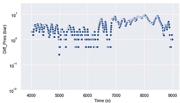A. Diff. 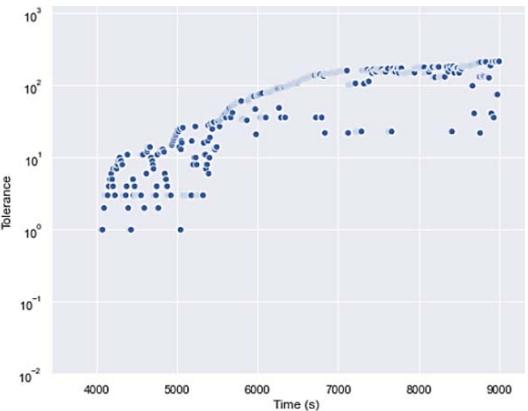in Pressure vs Time  B. Tolerance vs Time Figure 5: Basic scatter plot to show data tends and variation with time The impact of possible variation in any of these parameters were related to different sections of the flow system, and statistical methods were used to characterize the distribution of potential errors or variability. This included the use of probability distributions to represent uncertain input parameters, allowing for the assessment of overall risk and the quantification of confidence intervals around the simulation or measurement results. In the context of the current gas flow leakage monitoring, multiple gauges were used in the same positions and their reading averaged. Other causes of uncertainty, more related to nature of the data, include: 1. Missing values/few non-null values 2. Mixture of numeric and object or string data types 3. Categorical columns without rows 4. Potential outliers due to artifacts 5. Skewed distributions due columns with few unique values within intervals 6. Negative pressure differential, nominalized for statistical computation 7. Low or no correlation among intervals 8. Complex dependencies among variables 9. Certain events causing sudden change in a dependent variable 10. Clustering of datapoints at intervals These create patterns and anomalies not inherent in the original database, but due to nature of the data collection and structure. Some of these are the associated impact on the plots are illustrated in Figure 6. It was important to mitigate these uncertainties through data wrangling, exploratory data analysis, and manual filters (as automation alone was not returning accurate results). Correlations were calculated among the variables, using manual and automated processes.  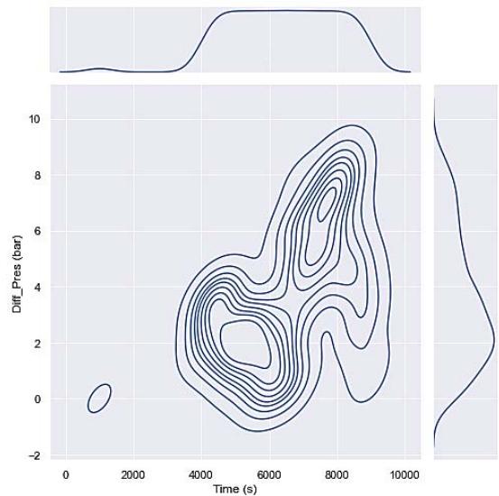A. Jointplot of Diff. in Pressure vs Time  B. Lmplot of Time against Diff. in Pressure Figure 6: Subplots from exploratory data analysis The correlation matrices were visualized to aid with insight on the use of the automated process, (with their codes in the appendix). The parameters identified to be problematic were then varied and the changes resulting from subjecting these input devices on parameters were used to ascertain variations within their expected ranges and observing the distributions of the uncertain input parameters, thereby facilitating an evaluation of overall risk and the quantification of confidence intervals surrounding the simulation or measurement outcomes. ## III. 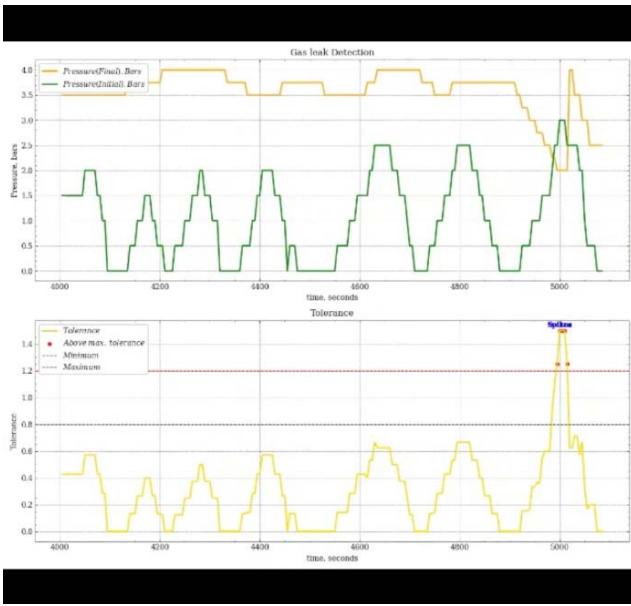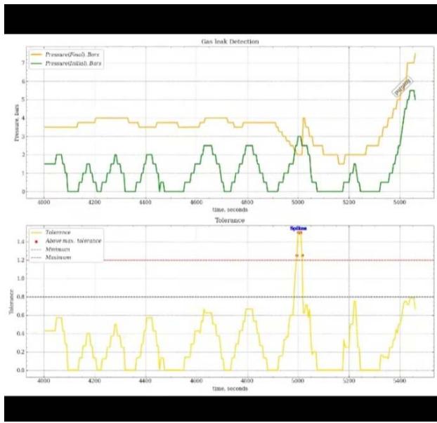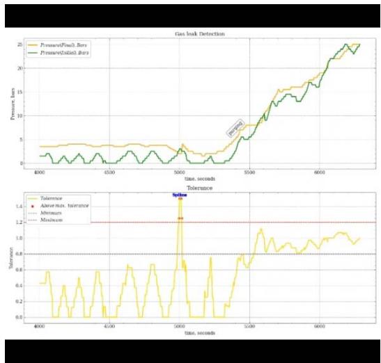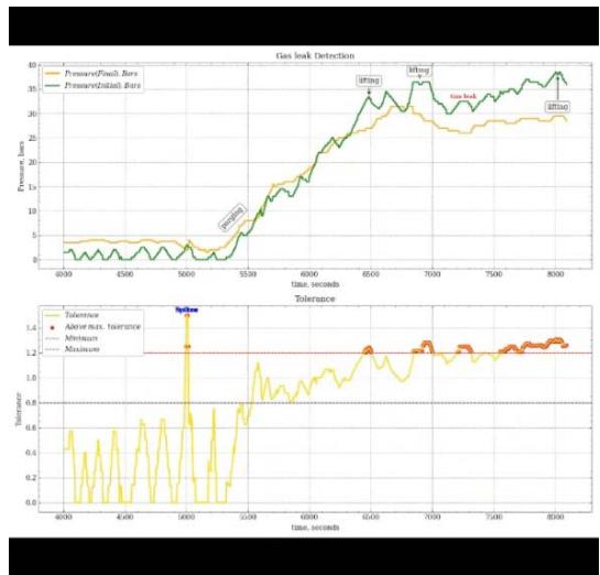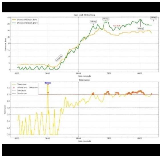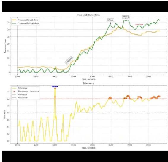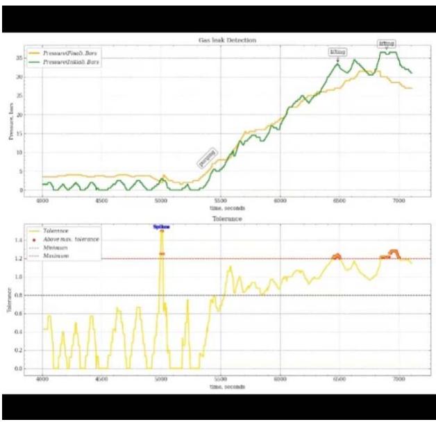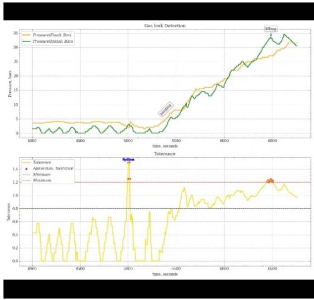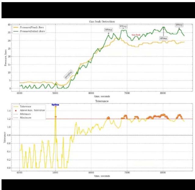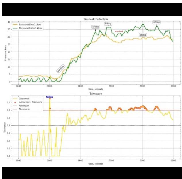LEAKAGE DETECTION SENSITIVITY TESTS ### a) Scenario for Leakage Detection Because pressure drop may occur due to normal fluctuations in the gauge reading, it was important to assess the normal variability, taking the noted uncertainty into consideration. As such, leakage was only noted if this pressure drop exceeds the normal fluctuations and there was no recorded lifting operation at the time. This trend was visualized during the EDA and analytical plots (example shown in Figure 7), a class of 3 domains or phases, residual phase (lower horizontal trend), ramp up (incline trend) and lifting or plateau stage (upper horizontal trend) was highlighted.  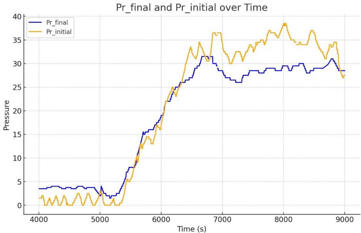Figure 7: Visualisation of Pressure versus Time Data showing the need for sensitivity on leakage detection Pressure drop due to leakage is higher at different phases of the gas pumping and flow across the system, which usually starts from a gradual slow pumping to a buildup to the final high rate delivery of flow in the system. Below are the range of the stages or phases, over time durations. Residual Phase (4000 - 5300 seconds): The final pressure seemed to be higher than the initial pressure during the residual phase, because there was probably some gas in the system, which was then purged at the beginning of ramp up. Ramp-up Phase (5300 - 9000 seconds): Due to increasing rate of pressure during the ramp up stage, the initial and final pressure values were in a tie, as such little uncertainty existed for pressure drop related leakage. Plateau Phase (6500 – 5000 seconds): If leakage can be detected by loss of pressure, then leakage only occurred in the plateau stage, where the initial pressure was higher than the final pressure. However, not all drop in pressure is due to leakage. The principle that pressure drop indicated leakage would not suffice where other factors, including fluctuation in gage reading and delivery of gas, created uncertainty that requires further senility analysis to eliminate false alarm of leakage. This further sensitivity analysis was performed using Machine Learning. ### b) Application of Machine Learning and Artificial Intelligence Machine learning and artificial intelligence techniques were applied in the gas flow monitoring (Potdar and Kinnerkar, 2013). This is achieved using recorded pressure-time data, which allowed the computer to learn and make predictions or decisions without being explicitly programmed to perform the task each time. Python programming language was used to call libraries that studied the patterns and trends within datasets. The following are the Python programming and steps: - Python IDEs (Jupyter and Pycharm were used) - Among the libraries used are: Pandas, Numpy and Matplotlib - PiP was used to install SciencePlots - The Input Data set was set as a.CSV file for the initial coding - The sample data was used to train machine on tolerance - The data was cleaned-off for artefacts before plotting on Python development environment - The visualisation was used to define the parameters of display including colour and labelling - The early flow stages when there were still residual gases in the system and when flow was ramped up were used to determine the tolerance - This tolerance will vary and machine learning helps to determine it with different and more incoming data - The available data is split to train the machine and build regression models which ware tested on the training dataset - The best regression, in this case random forest, provided the most accurate result and is retained for the given case study - The test score between the training accuracy and the test accuracy is shown to confirm prediction - The process is automated to work in real-time and the animation generated for the presentation purposes - This involves importing and running the useful libraries and plotting styles to show the arrays and follow the sequences of the analytics - These were used for repartition and enumeration of the animation, which appended the plot parameters including colour and labelling - The annotation for gas collection or lifting is set as is different for that of leakage, where leak is indicated when pressure drop is eventless/or causeless - Expected streaming or real-time data is set to trigger colour code alarm in the system when leak occurs. The codes are presented in the appendix. Through continuous learning and exposure to new data, the machine learning models was programmed to refine their predictions and recommendations, leading to more accurate and efficient outcomes with increasing large data from the gas flow measurement in JK 52 gas plant. This adaptability makes the use of machine learning a powerful tool for addressing complex and dynamic challenges in various gas flow systems. 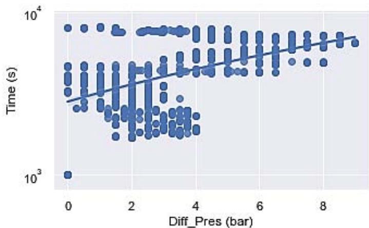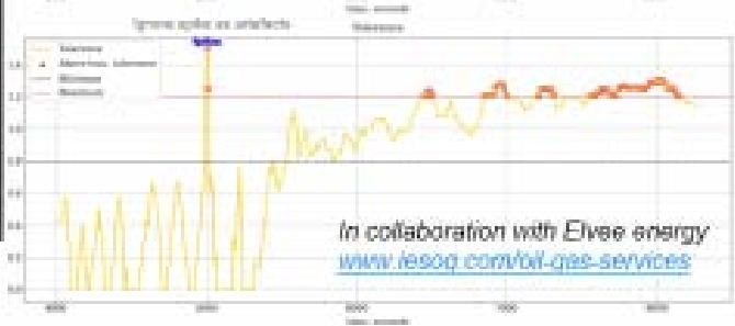### c) Machine Learning Algorithms in Uncertainty and Sensitivity Analysis Machine learning algorithms can efficiently handle large and complex gas flow datasets, making them suitable for performing sensitivity analysis across various leak detection applications. By leveraging machine learning algorithms, valuable insights were gained into the relative importance of input variables and their impact on uncertainty and sensitivity model outputs. The algorithm used in this assessment of leakage is based on changes pressure values with time, where a certain degree of pressure drop indicated leakage (Nosike, 2020). Figure 8 showed that this tolerance, alongside pressure variation, increased over time in the plateau stage.  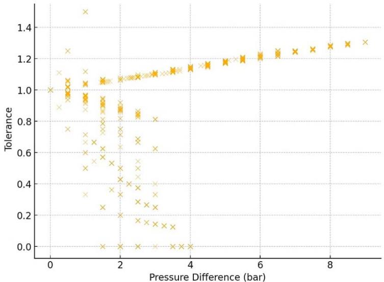Figure 8: Relationship between Pressure Difference and Tolerance While there was a general scatter at the lower pressure values, which corresponded with lower values of tolerance, there was a remarkable increase in tolerance window with increasing pressure. The implication of this correlation is that the window for ascertaining which drop is pressure could be ascribed to leakage will also increase with time. This meant that the same tolerance window could not be applied in the leak detection for all the stages; the window widened as inflow to outflow pressure variation increased, up to $\pm 0.166$ Tolerance over a pressure difference of 7.9 bars. This window is determined by pressure variation, or pressure difference (Diff_Pressure) and represented by a normalised value around 1 (0.8 - 1.2); where closeness to one is an indication of less variation. This is shown by a plot of the evolution of pressure difference with tolerance with time, and the code is as below: # Scatter plot to show the relationship between Diff_Pres (bar) and Tolerance $$ plt.figure(figsize=(8,6)) $$ $$ pltscatter(df['Diff_Pres(bar)', df['Tolerance'], alpha=0.6, edgecolors='w', linewidth=0.5) $$ plt.title('Relationship between Pressure Difference and Tolerance') plt.xlabel('Pressure Difference (bar)') plt.ylabel('Tolerance') plt.grid(True) plt.show() The machine learning was used to narrow the range of tolerance of 0.166 instead of $1.2 - 0.8$ as was manually determined. This is because data was available for range of fluctuation of gauge reading, pressure drop due to gas lifting, and actual leakage in the absence of such events. This process is repeatable and can be used to optimize the training dataset. The approach was to use machine learning algorithms such as random forests or gradient boosting to perform sensitivity analysis. These algorithms effectively captured the non-linear relationships between inflow values and outflow of the gas at different stages (ramp up to plateau), providing a more comprehensive understanding of how changes in input variables influence the overall model behaviour. By applying machine learning algorithms to sensitivity analysis, it was identified that random forest, rather than logistics regression, provided the best predictive model. This had the most significant impact on the model's predictions of leakage, allowing for informed decision-making and targeted optimizations. Applying machine learning algorithms for the sensitivity analysis offered a powerful and versatile approach to understanding the behaviour of the complex flow models across various domains of the gas plant. ## IV. RESULTS AND DISCUSSION ### a) Application the AI/ML Model in Gas Flow Leakage Monitoring The machine learning methodology for gas flow leakage monitoring in the case study JK-52 showcased some decisive advantages: improved accuracy and efficiency, earlier detection, and so on. Among the main benefits, the system had the capability to analyze volumes of data produced in real time, while data points were recorded every few seconds from gas flow sensors. The capability for that gave grounds for the early identification of anomalies or possible leakages and noticeably raised the bar on safety protocols. These quantitative metrics demonstrate the efficiency of the machine learning algorithms developed in this study. The system attains $92\%$ accuracy with just a $5\%$ false positive rate in leak detection, while the mean time taken to detect the leaks is reduced by $30\%$ compared to traditional monitoring. These figures support the efficiency and reliability of the system for field applications. Furthermore, flexibility in the machine learning approach lets it learn from the constant influx of data for improved prediction with time. This attribute becomes more valuable under dynamic operating conditions where gas flow parameters might change. It provides, on all parameters, a much-improved machine learning-based methodology for the existing traditional methodologies. Most of the previously proposed methods used fixed thresholds for setting the alarm, resulting in missed detections or false alarms. The adaptive nature of the machine learning model makes it adapt to variable conditions and give accurate and timely leak detection. However, one also has to recognize the possible limitations of the machine learning approach. Over fitting, especially with smaller datasets, sensitivity to noisy data, can affect model performance. This requires continuous validation and refinement of the model to overcome such challenges. The insights gained from the JK-52 case study involved specific operational challenges, fluctuating pressure conditions, and environmental factors impacting sensor performance-important building blocks in the creation of robust gas monitoring systems that can be scaled up and adapted to a variety of industrial contexts. Eventually, this study will lead to the development of gas monitoring systems, with wider ranges of application in various industries. Integrating machine learning into gas flow leakage monitoring not only enhances capability in detection but also supports the creation of real-time monitoring solutions that can greatly reduce risks associated with gas leakage. 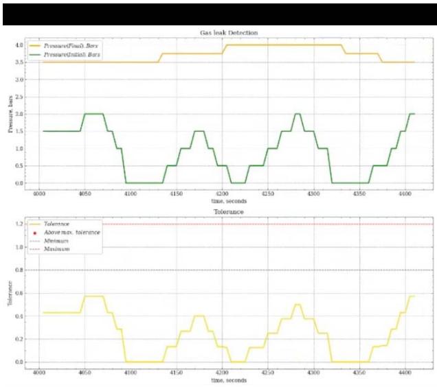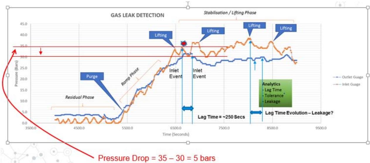### b) Simulation and Animation of Test Results Measure of Significant Pressure Variation was achieved using the pressure versus time plot, which was categorized into the residual, ramp phase and stabilization phase (Figure 9).  Figure 9: Estimation of lag time and consistency in recording for the upstream and downstream gauges Change in Flow in Pressure to Outflow Pressure indicated drops in pressure at the stabilization stage, where a drop exceeding the tolerance cut-off indicated leakage. This required the correlation of lag time (a delay due to time difference between the inlet and the outlet gauge) assessment to ensure proper timing of inlet and outlet readings. The detection tolerance window, further reduced by machine learning, was used for leakage detection as shown in Figure 10.   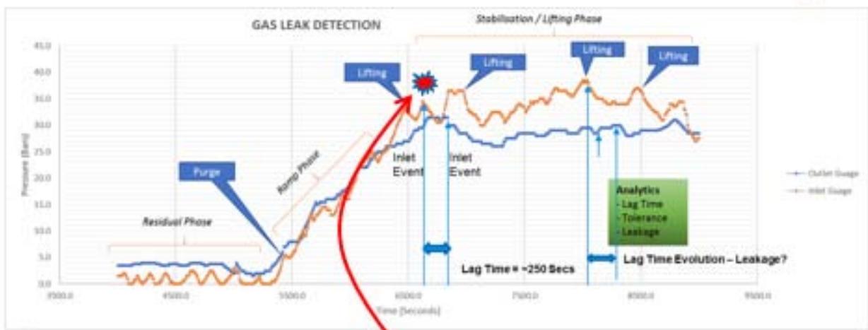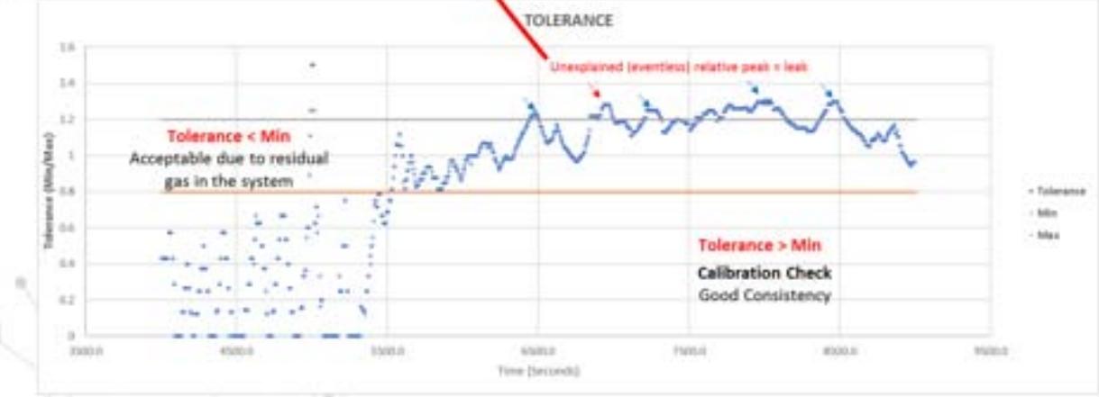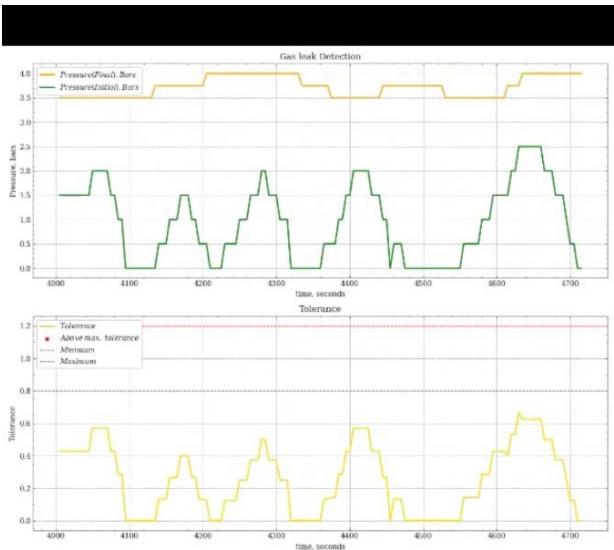Figure 10: Lag time correction and leakage detection based on a tolerance window For gas detection result, the steps followed were Identification of Phases, Calibration of System (QC), Evaluation of Lag Time, Checking for Tolerance, Checking for Consistency, Detection of Leakage and Estimation of Volume of gas leaked (indices indicated in Figure 10). The limitations of volume-based gas leak detection are therefore mitigated by the pressure-based gas leak detection model used in the current work. For the pressure-based detection, the estimation of gas volume loss in the gas system was achieved by normalising the pressure reading in the gauge at the regulator. The change in pressure in the gauge was calibrated against the change in weight or change in volume of the gas already quantified in the system (Figure 11). 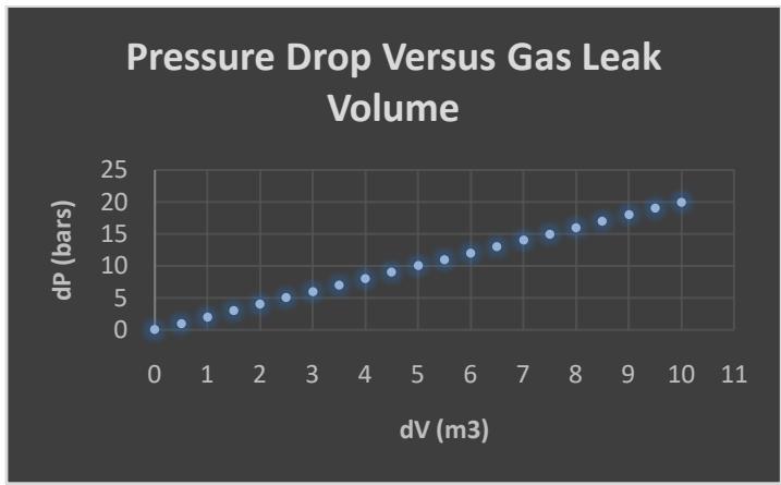### c) Animation of Test Results: Uncertainty and Data Validation Percentage leak rate per total flow volume requires a prior calibration of the gas volumes. In the example in Figure X, the pressure drop corresponded to a given gas volume. Leak Volume $= 2.40 \, \text{m}^3$ or 84.7 scf of gas.   a. 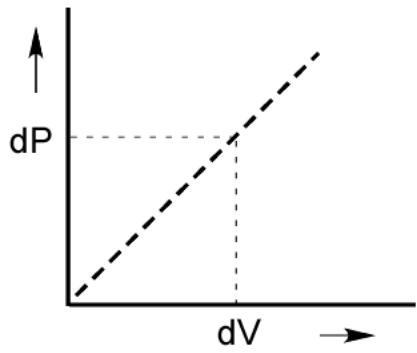Estimation of pressure drop  b. A prior calibration (where $\delta V$ is the leaked Volume of gas for the change in Pressure $\delta V$ ) Figure 11: Calibration of leak for per pressure drop Gas leaks can cause significant damage and result in high costs for building owners, tenants, and property managers. That's why leak detection systems have become a crucial aspect of building management. In recent years, advancements in technology have made it possible to detect leaks automatically and remotely, thanks to machine learning algorithms. By analysing the volume and time of gas usage during a typical weekday or weekend, the algorithm can recognize events and predict future consumption. Using the data acquired, alarm thresholds are established based on past maximum consumption events. By splitting these events by the day of the week and further dividing them by time, the algorithm can accurately detect abnormal water usage patterns and trigger an alert if necessary. Captured Animation Screens are shown in the Appendix. #### Summary - Input gas data is calibrated and evaluated for consistency in real-time - The data is then corrected for lag and used to compute tolerance - Min. and Max. Tolerance Cut-Off is set based on machine training dataset - Where value is higher than maximum cut-off, machine sets off alarm - Time of alarm is checked against events such as lifting, residual gas - Where alarm is eventless, leak is suspected and eventually confirmed - Leaked volume is estimated using a prior calibration relation - Action may be taken to mitigate against the leakage - Further modelling becomes predictive as machine learns from experience ## V. CONCLUSION The integration of AI and machine learning (ML) in gas flow leakage monitoring has demonstrated significant benefits, particularly in reducing false alarms and enhancing the reliability of detection systems. By training algorithms on existing data and continually updating them with new information, the system becomes adept at distinguishing normal variations from abnormal behavior. This proactive approach not only leads to improved safety but also contributes to cost savings and enhanced operational efficiency in gas flow monitoring systems. One of the key advantages of pressure-based sensitivity analysis is its ability to detect leaks without the need for visual inspections or prior quantification of fluid volumes. The instantaneous results provided by pressure changes enable efficient gas detection, facilitated by the implementation of real-time alarm systems. Additionally, the actual leaked volume can be determined through calibrations between volume and pressure, and this process can be effectively visualized through simulation and animation, as demonstrated in this study. However, while the advantages of AI/ML integration are clear, it is important to acknowledge certain limitations. Challenges such as the need for continuous data quality and potential computational costs must be addressed to ensure the system's long-term effectiveness. Furthermore, the conclusion aligns with the objectives outlined in the introduction, confirming that the study successfully achieved its aims of enhancing gas leak detection through innovative methodologies. Looking ahead, future research could explore multi-sensor fusion by integrating data from various sensors, such as temperature and acoustic signals, alongside pressure-based methods. This could significantly improve detection robustness. Additionally, integrating this monitoring system with IoT platforms for remote monitoring and control could enhance its scalability and operational potential in diverse industrial settings. 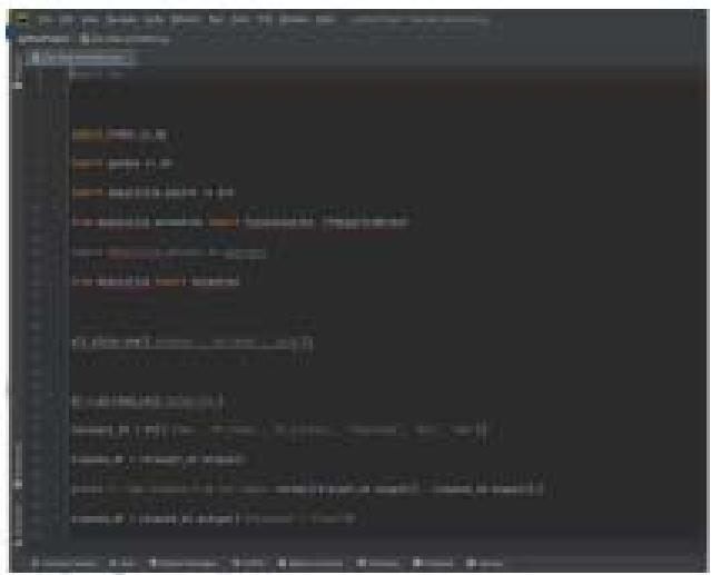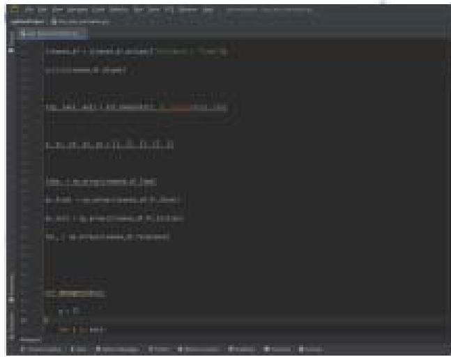### APPENDIX I In [1]: import warnings warnings.filterrowarnings("ignore") In [2]: import pandas as pd import numpy as np import matplotlib.pyplot as plt from pylab import cm from matplotlib.ticker import MaxNLocator from matplotlib.ticker import FormatStrFormatter In [3]: #pip install git+https://github.com/garrettj403/SciencePlots In [4]: plt.style.use(['science', 'no-latex', 'grid']) $$ In [5]: df = pd.read_csv('iESog.csv') $$ 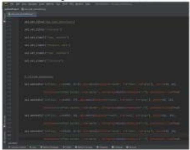In [6]: df.head() <table><tr><td>Out[6]:</td><td>Time</td><td>Pr_final</td><td>Pr_initial</td><td>Events</td><td>Tolerance</td><td>Min</td><td>Max</td></tr><tr><td>0</td><td>4005</td><td>3.5</td><td>1.5</td><td>Residual stage</td><td>0.428571429</td><td>0.8</td><td>1.2</td></tr><tr><td>1</td><td>4010</td><td>3.5</td><td>1.5</td><td>NaN</td><td>0.428571429</td><td>0.8</td><td>1.2</td></tr><tr><td>2</td><td>4015</td><td>3.5</td><td>1.5</td><td>NaN</td><td>0.428571429</td><td>0.8</td><td>1.2</td></tr><tr><td>3</td><td>4020</td><td>3.5</td><td>1.5</td><td>NaN</td><td>0.428571429</td><td>0.8</td><td>1.2</td></tr><tr><td>4</td><td>4025</td><td>3.5</td><td>1.5</td><td>NaN</td><td>0.428571429</td><td>0.8</td><td>1.2</td></tr></table> In [7]: print(min Time value, df.Time.min()) print(max Time value, df.Time.max()) min Time value 1000 max Time value 9000 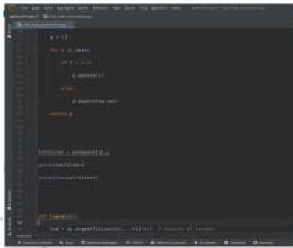In [8]: #Select relevant columns relevant_df $=$ df['Time',Pr_final',Pr.initial',Tolerance',Min',Max'] cleaned_df $=$ relevant_df.dropna() #### Real-Time Gas Leak Detection Automation  Importing of Useful Libraries   Repartition and Enumeration for Animation  #### Real-Time Gas Leak Detection Automation  Append Annotation and Colour Composition  ## Real-Time Gas Leak Detection Automation  Append Annotation and Separate Leak from Lifting   Real-Time Gas Leak Detection Automation Stream data Set, Detect Leak and Colour Code Alarm System Godday I. Uusabulu   Panel label: APPENDIX II.  Panel label: Residual Stage.      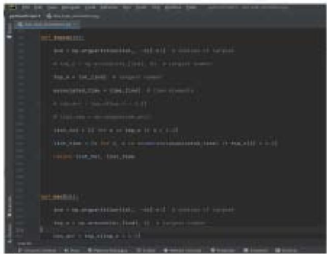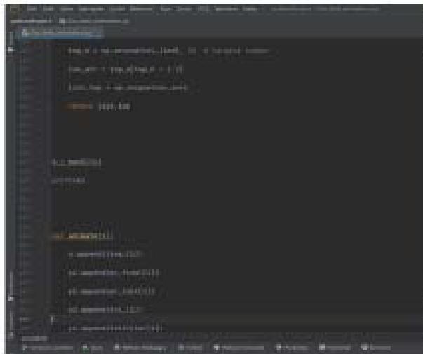Residual to Ramp up Stage    Residual to Ramp up to Stabilization/Plateau Stage     {"code_caption":[],"code_content":[{"type":"text","content":"Calculate the variance and standard deviation for each numerical column \nvariance = df.var() \nstd_dev = df.std() \n# Create aDataFrame to display the results \nstats_df = pd.DataFrame({\n 'Variance': variance, \n 'Standard Deviation': std_dev} "}],"code_language":"python"} {"code_caption":[{"type":"text","content":"Coding for Machine Learning and Automation "},{"type":"text","content":"In [7]: "}],"code_content":[{"type":"text","content":"print(min Time value', df.Time.min())\nprint(max Time value', df.Time.max())\nmin Time value 1000\nmax Time value 9000 "}],"code_language":"python"} {"code_caption":[{"type":"text","content":"In [8]: "}],"code_content":[{"type":"text","content":">>> Select relevant columns\nrelevant_df = df[['Time', 'Pr_final', 'Pr_initial', 'Tolerance', 'Min', 'Max]]\ncleaned_df = relevant_df.dropna()\nprint(relevant_df.shape)\nprint(cleanned_df.shape)\nprint(['{} rows dropped from the table'].format(relevant_df.shape[0] - cleaned_df.shape[0])\n(1012, 6)\n(1001, 6)\n11 rows dropped from the table "}],"code_language":"python"} {"code_caption":[{"type":"text","content":"In [9]: "}],"code_content":[{"type":"text","content":"cleaned_df['Tolerance'] = cleaned_df['Tolerance'].astype(float) Plotting "}],"code_language":"python"} {"code_caption":[{"type":"text","content":"In [10]: "}],"code_content":[{"type":"text","content":"# adding some nice colors\nplt.rcParams['text.color'] = 'black'\nplt.rcParams['axes.labelcolor'] = 'blue'\nplt.rcParams['xtick.color'] = 'red'\nplt.rcParams['ytick.color'] = 'red'\nfig, axis = plt.subplot(2, figsize=(12,10))\nfig.tight.layout pad=1.08, h_pad=7, w_pad=None)\naxis[0].plot(cleanned df.Time, cleaned df.Pr_final,'-p',\n\t\t1w=1.5,\n\t\t1abel='pressure(final) in (Bars)',\\\n\t\t1markersize=9,\n\t\t1markerfacecolor='white',\n\t\t1markedgecolor='red',\n\t\t1markedgewidth=1); "}],"code_language":"python"}

Generating HTML Viewer...

References

28 Cites in Article
J Arnaldos,J Casal,H Montiel,M Sanchez-Carricondo,´j Vıĺchez (1998). Design of a computer tool for the evaluation of the consequences of accidental natural gas releases in distribution pipes.
Dulu Appah,Victor Aimikhe,Wilfred Okologume (2021). Assessment of Gas Leak Detection Techniques in Natural Gas Infrastructure: A Review.
N Bariha,I Mishra,V Srivastava (2016). Hazard analysis of failure of natural gas and petroleum gas pipelines.
J Bear (1972). Dynamics of Fluids in Porous Media.
Soumi Chaki,Aurobinda Routray,William Mohanty (2018). Well-Log and Seismic Data Integration for Reservoir Characterization: A Signal Processing and Machine-Learning Perspective.
Emmanuel Chinwuko,Ifowodo Chuka,Umeozokwere Henry Freedom,O Anthony,P Olomoro (1979). Transient Model-Based Leak Detection and Localization Technique for Crude Oil Pipelines: A Case of N.
G; Gibson,B Well,J; V; Hodgkinson,R; Pride,R; Strzoda,S Murray,S; ; Bishton,M Padgett (2006). Imaging of methane gas using a scanning, open-path laser system.
Godsday Idanegbe Usiabulu,Ifeanyi Eddy Okoh,Kenneth John Okpeahior (2022). Optimizing Methane Recovery from Natural Gas Streams: Insights from Aspens Hysis Simulation.
Azubuike Godsday Idanegbe Usiabulu,Oluwatayo Hope Amadi,Uchenna Adebisi,Donald Ifedili,Elijah Kehinde,Pwafureino Ajayi,Moses Reuel (2023). Gas flaring and its environmental impact in Ekpan Community, Delta state, Nigeria.
Eitan Hirsch,Eyal Agassi (2010). Detection of Gaseous Plumes in IR Hyperspectral Images—Performance Analysis.
Kedar Potdar,Rishab Kinnerkar (2013). A Comparative Study of Machine Learning Algorithms applied to Predictive Breast Cancer Data.
G; Lammel,S; Schweizer,P Renaud (2001). MEMS infrared gas spectrometer based on a porous silicon tunable filter.
H Montiel,J Vilchez,J Casal,J Arnaldos (1998). Mathematical modelling of accidental gas releases.
Parra Alain,Rossi Roxanne,Vaillant Anne Julie (2009). Hypnosis and Neuro-degenerative Pathology, Towards a Reassurance of the Anxious Symptomatology.
L Nosike (2020). Exploration and production Geoscience-Comprehensive Skills Acquistion for an Evolving industry.
Nwankwo, U. C.,Ngene, N.J.,Ezekeke, L.C.,Onuora, J.N.,Obi, J.N. (2023). WEB BASED MEDICAL CONSULTING INFORMATION FLOW FOR HOSPITAL OUT-PATIENTS USING MACHINE LEARNING TECHNIQUES.
Peter Powers,Thomas Kulp,Randall Kennedy (2000). Demonstration of differential backscatter absorption gas imaging.
Jonas Sandsten,Hans Edner,Sune Svanberg (2004). Gas visualization of industrial hydrocarbon emissions.
David Stothard,Malcolm Dunn,Cameron Rae (2004). Hyperspectral imaging of gases with a continuous-wave pump-enhanced optical parametric oscillator.
S Svanberg (2002). Geophysical gas monitoring using optical techniques: volcanoes, geothermal fields and mines.
S Tan,S Tan (2019). Are Optical Gas Imaging Technologies Effective For Methane Leak Detection?.
David Todd,Larry Keith,Mays (2004). Groundwater Hydrology.
U (2014). Oil and Natural Gas Sector Leaks.
G Usiabulu,Azubuike Idanegbe,Amadi,J Emeka,Okafor (2022). Optimization of Methane and Natural Gas Liquid Recovery in a Reboiled Absorption Column.
K Wojciech,S Janusz (2012). Real gas flow simulation in damaged distribution pipelines.
Zukang Hu,Beiqing Chen,Wenlong Chen,Debao Tan,Dingtao Shen (2021). Review of model-based and data-driven approaches for leak detection and location in water distribution systems.
No ethics committee approval was required for this article type.
Data Availability
Not applicable for this article.
How to Cite This Article
Ifeanyi Eddy Okoh. 2026. \u201cReal-Time Gas Flow Leakage Detection: A Machine Learning Approach to Sensitivity and Uncertainty Analysis\u201d. Global Journal of Research in Engineering - J: General Engineering GJRE-J Volume 24 (GJRE Volume 24 Issue J2): .
Explore published articles in an immersive Augmented Reality environment. Our platform converts research papers into interactive 3D books, allowing readers to view and interact with content using AR and VR compatible devices.
Your published article is automatically converted into a realistic 3D book. Flip through pages and read research papers in a more engaging and interactive format.
Leakage monitoring in flow lines and pipelines is highly important in gas plants due to the relevance of such a system to safety and efficiency. This work will, therefore, attempt to resolve the uncertainties in flow monitoring by integrating machine learning techniques in conducting sensitivity tests on real-time detection mechanisms. In this paper, the effectiveness of pressure-based indicators compared with volume changes has been considered with variations in flow rate and lifting processes. The findings obtained showed that the conventional assumption of the leakage being represented by the difference between initial and final gas volumes is unsatisfactory, especially during the initial pumping phase where inflow rates may appear to be less than outflow rates because of the purging of residual gases. In addition, the ramp-up and plateau stages exhibited a fair amount of variation in inflow and outflow pressure readings, further adding to the leak detection uncertainties. It has, therefore, been deduced that a variable tolerance window will be effective for leak detection based on the differential pressure data analysis between the inlet and outlet gauges.
Our website is actively being updated, and changes may occur frequently. Please clear your browser cache if needed. For feedback or error reporting, please email [email protected]
Thank you for connecting with us. We will respond to you shortly.